Designing R functions to compute betadiversity indices from species lists
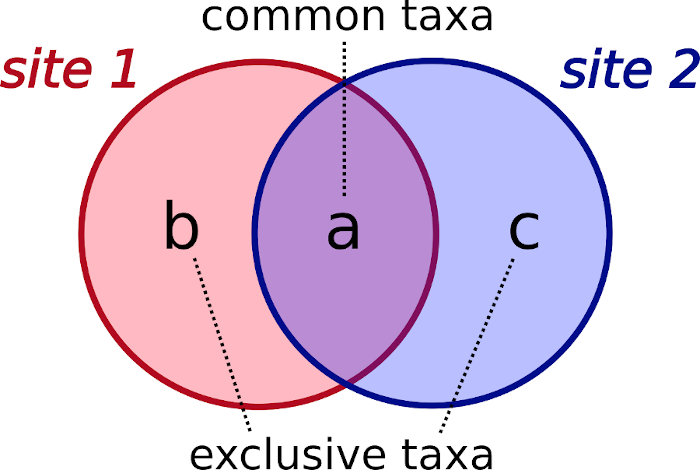 Image credit: Blas M. Benito
We ecologists like to measure all things in nature, and compositional changes in biological communities over time or space, a.k.a betadiversity, is one of these things. I am not going to explain what betadiversity is because others that know better than me have done it already. Good examples are this post published the blog of Methods in Ecology and Evolution by Andres Baselga, and this lecture by Tim Seipel.
What I am actually going to do in this post is to explain how to write functions to compute betadiversity indices in R from species lists rather than from presence-absence matrices. For the latter there are a few packages such as vegan, BAT, MBI, or betapart, but for the former I was unable to find anything suitable. To make this post useful for R beginners, I will go step by step on the rationale behind the design of the functions to compute betadiversity indices, and by the end of the post I will explain how to organize them to achieve a clean R workflow.
Let’s go!
Betadiversity indices
There are a few betadiversity indices out there, and I totally recommend you to start with Koleff et al. (2003) as a primer. They review the literature and analyze the properties of 24 different indices to provide guidance on how to use them.
Betadiversity components a, b, and c
Betadiversity indices are designed to compare the taxa pools of two sites at a time, and require the computation of three components:
- a: number of common taxa of both sites.
- b: number of exclusive taxa of one site.
- c: number of exclusive taxa of the other site.
Let’s see how can we use these diversity components to compute betadiversity indices.
Sørensen’s Beta
Let’s start with the Sørensen’s Beta (\(\beta_{sor}\) hereafter), as presented in Koleff et al. (2003).
\[\beta_{sor} = \frac{2a}{2a + b + c}\]
\(\beta_{sor}\) is a similarity index in the range [0, 1] (the closer to one, the more similar the taxa pools of both sites are) that puts a lot of weight in the \(a\) component, and is therefore a measure of continuity, as it focuses the most in the common taxa among sites.
Simpson’s Beta
Another popular betadiversity index is the Simpson’s Beta (\(\beta_{sim}\) hereafter).
\[\beta_{sim} = \frac{min(b, c)}{min(b, c) + a}\] where \(min()\) is a function that takes the minimum value among the diversity components within the parenthesis. \(\beta_{sim}\) is a dissimilarity measure that focuses on compositional turnover among sites because it focuses the most on the values of \(b\) and \(c\). It has its lower bound in zero, and an open upper value.
To bring these ideas into R, first we have to load a few R packages, and generate some fake data to help us develop the functions.
library(magrittr)
library(foreach)
library(doParallel)
## Loading required package: iterators## Loading required package: parallelThe code chunk below generates 15 fake taxa names, from taxon_1 to taxon_15.
taxa <- paste0("taxon_", 1:15)With these fake taxa we are going to generate taxa lists for four hypothetical sites named site1, site2, site3, and site4. Two of the sites will have identical taxa lists, two will have non-overlapping taxa lists, and two of them will have some overlap.
site1 <- site2 <- taxa[1:7]
site3 <- taxa[8:12]
site4 <- taxa[10:15]
So now we have these taxa lists:
site1 #and site2## [1] "taxon_1" "taxon_2" "taxon_3" "taxon_4" "taxon_5" "taxon_6" "taxon_7"site3## [1] "taxon_8" "taxon_9" "taxon_10" "taxon_11" "taxon_12"site4## [1] "taxon_10" "taxon_11" "taxon_12" "taxon_13" "taxon_14" "taxon_15"
Step-by-step computation of betadiversity indices with R
For a given pair of sites, how can we compute the diversity components a, b, and c?
Looking at it from an R perspective, each site is a character vector, so a can be found by counting the number of common elements between two vectors. These common elements can be found with the function intersect(), and the number of elements can be computed by applying length() on the result of intersect().
a <- length(intersect(site3, site4))
a
## [1] 3To compute b and c we can use the function setdiff(), that finds the exclusive elements of one character vector when comparing it with another. In this case, b is computed for the first vector introduced in the function, site3 in this case…
b <- length(setdiff(site3, site4))
b
## [1] 2… so to compute the c component we only need to switch the sites.
c <- length(setdiff(site4, site3))
c
## [1] 3Now that we know a, b, and c, we can compute \(\beta_{sor}\) and \(\beta_{sim}\).
Bsor <- 2 * a / (2 * a + b + c)
Bsor
## [1] 0.5454545Bsim<- min(b, c) / (min(b, c) + a)
Bsim## [1] 0.4Of course, if we have a long list of sites, computing betadiversity indices like this can get quite boring quite fast. Let’s put everything in a set of functions to make it easier to work with.
Writing functions to compute betadiversity indices
The basic structure of a function definition in R looks as follows:
function_name <- function(x, y, ...){
  output <- [body]
  output #also return(output)
}
Where:
function_nameis the name of your function. Ideally, a verb, or otherwise, something indicating somehow what the function will do with the input data and arguments.function()is a function to define functions, there isn’t much more to it…xis the first argument of the function, and ideally, represents the input data. If that is the case, you can later use pipes (%>%) to chain functions together.y(it could have any other name) is another function argument, an can be either another input dataset, or an argument defining how the function has to behave....refers to other arguments the function may require.bodyis the code that operates with the data and function arguments. This can be one line of code, or a thousand, it all comes down to the function’s objective. In any case, thebodymust return an object (or an error if something went wrong) that will be the function’soutput.outputis the object ultimately produced by the function. It can have any name, and can be any kind of structure, such a number, a vector, a data frame, a list, etc. R functions return one output object only. Since R functions return the last evaluated value, it is good practice to put theoutputobject at the end of the function as an explicit way to state what the actual output of the function is.
Let’s start writing a function to compute a, b, and c from a pair of sites.
#x: taxa list of one site
#y: taxa list of another site
abc <- function(x, y){

  #list to store output
  out <- list()

  #filling the list
  out$a <- length(intersect(x, y))
  out$b <- length(setdiff(x, y))
  out$c <- length(setdiff(y, x))

  #returning the output
  out
}
Notice that to to return the three values I am wrapping them in a list. Let’s run a little test.
x <- abc(
  x = site3,
  y = site4
)
x
## $a
## [1] 3
##
## $b
## [1] 2
##
## $c
## [1] 3So far so good! From here we build the functions sorensen_beta() and simpson_beta() making sure they can accept the output of abc(), and return it with an added slot.
sorensen_beta <- function(x){

  x$bsor <- round(2 * x$a / (2 * x$a + x$b + x$c), 3)

  x

}


simpson_beta <- function(x){

  x$bsim <- round(min(x$b, x$c) / (min(x$b, x$c) + x$a), 3)

  x

}
Notice that both functions are returning the input x with an added slot named after the given betadiversity index. Let’s test them first, to later see why returning the input object gives these functions a lot of flexibility.
sorensen_beta(x)## $a
## [1] 3
##
## $b
## [1] 2
##
## $c
## [1] 3
##
## $bsor
## [1] 0.545simpson_beta(x)## $a
## [1] 3
##
## $b
## [1] 2
##
## $c
## [1] 3
##
## $bsim
## [1] 0.4When I said that returning the input object with an added slot gave these functions a lot of flexibility I was talking about this:
x <- abc(
  x = site3,
  y = site4
  ) %>%
  sorensen_beta() %>%
  simpson_beta()
x
## $a
## [1] 3
##
## $b
## [1] 2
##
## $c
## [1] 3
##
## $bsor
## [1] 0.545
##
## $bsim
## [1] 0.4Chaining the functions through the %>% pipe of the magrittr package now allows us to combine their results in a single output no matter whether we use sorensen_beta() or sorensen_beta() first, or whether we omit one of them. The only thing the pipe is doing here is moving the output of the first function into the next. There are a couple of very nice tutorials about the magrittr package and the %>% here and here.
We can put that idea right away into a function to compute both betadiversity indices at once from the taxa list of a pair of sites.
betadiversity <- function(x, y){

  require(magrittr)

  abc(x, y) %>%
    sorensen_beta() %>%
    simpson_beta()

}
The function now works as follows.
x <- betadiversity(
  x = site3,
  y = site4
  )
x
## $a
## [1] 3
##
## $b
## [1] 2
##
## $c
## [1] 3
##
## $bsor
## [1] 0.545
##
## $bsim
## [1] 0.4So far we have four functions…
abc()simpson_beta(), that requiresabc().sorensen_beta(), that requiresabc().betadiversity(), that requiresabc(),simpson_beta(), andsorensen_beta().
… and one limitation: so far we can only return betadiversity indices for two sites at a time. So at the moment, to compute betadiversity indices for all combinations of sites we have to do a pretty ridiculous thing:
x1 <- betadiversity(x = site1, y = site2)
x2 <- betadiversity(x = site1, y = site3)
x3 <- betadiversity(x = site1, y = site4)
#... and so on
If I see you doing this I’ll come to haunt you in your nightmares! Since a real analysis may involve hundreds of sites, the next step is to use the functions above to build a new one able to intake an arbitrary number of sites.
Writing a function to compute betadiversity indices for an arbitrary number of sites.
First we have to organize our sites in a data frame with a long format.
sites <- data.frame(
  site = c(
    rep("site1", length(site1)),
    rep("site2", length(site2)),
    rep("site3", length(site3)),
    rep("site4", length(site4))
    ),
  taxon = c(
    site1,
    site2,
    site3,
    site4
  )
)| site | taxon |
|---|---|
| site1 | taxon_1 |
| site1 | taxon_2 |
| site1 | taxon_3 |
| site1 | taxon_4 |
| site1 | taxon_5 |
| site1 | taxon_6 |
| site1 | taxon_7 |
| site2 | taxon_1 |
| site2 | taxon_2 |
| site2 | taxon_3 |
| site2 | taxon_4 |
| site2 | taxon_5 |
| site2 | taxon_6 |
| site2 | taxon_7 |
| site3 | taxon_8 |
| site3 | taxon_9 |
| site3 | taxon_10 |
| site3 | taxon_11 |
| site3 | taxon_12 |
| site4 | taxon_10 |
| site4 | taxon_11 |
| site4 | taxon_12 |
| site4 | taxon_13 |
| site4 | taxon_14 |
| site4 | taxon_15 |
Our new function will need to do several things:
- Generate combinations of the unique values of the column
sitetwo by two without repetition. - Iterate through these combinations of two sites to compute betadiversity components and indices.
- Return a dataframe with the results to facilitate further analyses.
The combinations of site pairs are done with utils::combn() as follows:
site.combinations <- utils::combn(
  x = unique(sites$site),
  m = 2
  )
site.combinations
## [,1] [,2] [,3] [,4] [,5] [,6]
## [1,] "site1" "site1" "site1" "site2" "site2" "site3"
## [2,] "site2" "site3" "site4" "site3" "site4" "site4"The result is a matrix, and each pair of rows in a column contain a pair of sites. The idea now is to iterate over the matrix columns, obtain the set of taxa from each site from the taxon column of the sites data frame, and use these taxa lists to compute the betadiversity components and indices.
To easily generate the output data frame, I use the foreach::foreach() function to iterate through pairs instead of a more traditional for loop. You can read more about foreach() in a previous post.
betadiversity.df <- foreach::foreach(
  i = 1:ncol(site.combinations), #iterates through columns of site.combinations
  .combine = 'rbind' #to produce a data frame
  ) %do% {

  #site names
  site.one <- site.combinations[1, i] #from column i, row 1
  site.two <- site.combinations[2, i] #from column i, row 2

  #getting taxa lists
  taxa.list.one <- sites[sites$site %in% site.one, "taxon"]
  taxa.list.two <- sites[sites$site %in% site.two, "taxon"]

  #betadiversity
  beta <- betadiversity(
    x = taxa.list.one,
    y = taxa.list.two
  )

  #adding site names
  beta$site.one <- site.one
  beta$site.two <- site.two

  #returning output
  beta

}| a | b | c | bsor | bsim | site.one | site.two |
|---|---|---|---|---|---|---|
| 7 | 0 | 0 | 1 | 0 | site1 | site2 |
| 0 | 7 | 5 | 0 | 1 | site1 | site3 |
| 0 | 7 | 6 | 0 | 1 | site1 | site4 |
| 0 | 7 | 5 | 0 | 1 | site2 | site3 |
| 0 | 7 | 6 | 0 | 1 | site2 | site4 |
| 3 | 2 | 3 | 0.545 | 0.4 | site3 | site4 |
Now that we know it works, we can put everything together in a function. Notice that to make the function more general, I have added arguments requesting the names of the columns with the site and the taxa names.
betadiversity_multisite <- function(
  x,
  site.column, #column with site names
  taxa.column #column with taxa names
){

  #get site combinations
  site.combinations <- utils::combn(
    x = unique(x[, site.column]),
    m = 2
  )

  #iterating through site pairs
  betadiversity.df <- foreach::foreach(
    i = 1:ncol(site.combinations),
    .combine = 'rbind'
  ) %do% {

    #site names
    site.one <- site.combinations[1, i]
    site.two <- site.combinations[2, i]

    #getting taxa lists
    taxa.list.one <- x[x[, site.column] %in% site.one, taxa.column]
    taxa.list.two <- x[x[, site.column] %in% site.two, taxa.column]

    #betadiversity
    beta <- betadiversity(
      x = taxa.list.one,
      y = taxa.list.two
    )

    #adding site names
    beta$site.one <- site.one
    beta$site.two <- site.two

    #returning output
    beta

  }

  #remove bad rownames
  rownames(betadiversity.df) <- NULL

  #reordering columns
  betadiversity.df <- betadiversity.df[, c(
    "site.one",
    "site.two",
    "a",
    "b",
    "c",
    "bsor",
    "bsim"
    )]

  #returning output
  return(betadiversity.df)

}
And the test!
sites.betadiversity <- betadiversity_multisite(
  x = sites,
  site.column = "site",
  taxa.column = "taxon"
)| site.one | site.two | a | b | c | bsor | bsim |
|---|---|---|---|---|---|---|
| site1 | site2 | 7 | 0 | 0 | 1 | 0 |
| site1 | site3 | 0 | 7 | 5 | 0 | 1 |
| site1 | site4 | 0 | 7 | 6 | 0 | 1 |
| site2 | site3 | 0 | 7 | 5 | 0 | 1 |
| site2 | site4 | 0 | 7 | 6 | 0 | 1 |
| site3 | site4 | 3 | 2 | 3 | 0.545 | 0.4 |
That went well!
Finally, to have these functions available in my R session I always put them all in a single file in the same folder where my Rstudio project lives, name it something like functions_betadiversity.R, and source it at the beginning of my script or .Rmd file by running a line like the one below.
source("functions_betadiversity.R")I have placed the file functions_betadiversity.R in this GitHub Gist in case you want to give it a look. You can also source it right away to your R environment by executing the following line:
source("https://gist.githubusercontent.com/BlasBenito/4c3740b056a0c9bb3602f33dfd35990c/raw/bbb40d868787fc5d10e391a2121045eb5d75f165/functions_betadiversity.R")I hope this post helped you to better understand how to write and organize R functions!