Mapping Categorical Predictors to Numeric With Target Encoding
 Target encoding of a toy data frame performed with collinear::target_encoding_lab()
Summary
Categorical predictors are annoying stringy monsters that can turn any data analysis and modeling effort into a real annoyance. The post delves into the complexities of dealing with these types of predictors using methods such as one-hot encoding (please don’t) or target encoding, and provides insights into its mechanisms and quirks
Key Highlights:
-
Categorical Predictors are Kinda Annoying: This section discusses the common issues encountered with categorical predictors during data analysis.
-
One-Hot Encoding Pitfalls: While discussing one-hot encoding, the post focuses on its limitations, including dimensionality explosion, increased multicollinearity, and sparsity in tree-based models.
-
Intro to Target Encoding: Introducing target encoding as an alternative, the post explains its concept, illustrating the basic form with mean encoding and subsequent enhancements with additive smoothing, leave-one-out encoding, and more.
-
Handling Sparsity and Repetition: It emphasizes the potential pitfalls of target encoding, such as repeated values within categories and their impact on model performance, prompting the exploration of strategies like white noise addition and random encoding to mitigate these issues.
-
Target Encoding Lab: The post concludes with a detailed demonstration using the
collinear::target_encoding_lab()function, offering a hands-on exploration of various target encoding methods, parameter combinations, and their visual representations.
The post intends to serve as a useful resource for data scientists exploring alternative encoding techniques for categorical predictors.
Resources
- Interactive notebook of this post.
- A preprocessing scheme for high-cardinality categorical attributes in classification and prediction problems
- Extending Target Encoding
- Target encoding done the right way.
R packages
This tutorial requires the development version (>= 1.0.3) of the newly released R package
collinear, and a few more.
#required
install.packages("remotes")
remotes::install_github(
  repo = "blasbenito/collinear",
  ref = "development",
  force = TRUE
  )
install.packages("fastDummies")
install.packages("rpart")
install.packages("rpart.plot")
install.packages("dplyr")
install.packages("ggplot2")
library(rpart)
library(rpart.plot)
library(collinear)
library(fastDummies)
## Thank you for using fastDummies!
## To acknowledge our work, please cite the package:
## Kaplan, J. & Schlegel, B. (2023). fastDummies: Fast Creation of Dummy (Binary) Columns and Rows from Categorical Variables. Version 1.7.1. URL: https://github.com/jacobkap/fastDummies, https://jacobkap.github.io/fastDummies/.
library(dplyr)
##
## Attaching package: 'dplyr'
## The following objects are masked from 'package:stats':
##
##     filter, lag
## The following objects are masked from 'package:base':
##
##     intersect, setdiff, setequal, union
library(ggplot2)
Categorical Predictors are Kinda Annoying
I mean, the title of this section says it already, and I bet you have experienced it during an Exploratory Data Analysis (EDA) or a feature selection for model training and the likes. You likely had a nice bunch of numerical variables to use as predictors, no issues there. But then, you discovered among your columns thingies like “sampling_location”, “region_name”, “favorite_color”, or any other type of predictor made of strings, lots of strings. And some of these made sense, and some of them didn’t, because who knows where they came from. And you had to branch your code to deal with numeric and categorical variables separately. Or maybe chose to ignore them, as I have done plenty of times.
Yeah, nobody likes them much at all, But sometimes, these stringy monsters are all you have to move on with your work. And you are not the only one. That’s why many efforts have been made to convert them to numeric and kill the problem at once, so now we all have two problems instead.
Let me go ahead and illustrate the issue. There is a nice data frame in the collinear R package named vi, with one response variable named vi_mean, and several numeric and categorical predictors named in the vector vi_predictors.
data(
  vi,
  vi_predictors
)

dplyr::glimpse(vi)
## Rows: 30,000
## Columns: 68
## $ longitude                  <dbl> -114.254306, 114.845693, -122.145972, 108.3…
## $ latitude                   <dbl> 45.0540272, 26.2706940, 56.3790272, 29.9456…
## $ vi_mean                    <dbl> 0.38, 0.53, 0.45, 0.69, 0.42, 0.68, 0.70, 0…
## $ vi_max                     <dbl> 0.57, 0.67, 0.65, 0.85, 0.64, 0.78, 0.77, 0…
## $ vi_min                     <dbl> 0.12, 0.41, 0.25, 0.50, 0.25, 0.48, 0.60, 0…
## $ vi_range                   <dbl> 0.45, 0.26, 0.40, 0.34, 0.39, 0.31, 0.17, 0…
## $ vi_binary                  <dbl> 0, 1, 0, 1, 0, 1, 1, 0, 1, 0, 0, 1, 0, 0, 0…
## $ koppen_zone                <chr> "BSk", "Cfa", "Dfc", "Cfb", "Aw", "Cfa", "A…
## $ koppen_group               <chr> "Arid", "Temperate", "Cold", "Temperate", "…
## $ koppen_description         <chr> "steppe, cold", "no dry season, hot summer"…
## $ soil_type                  <chr> "Cambisols", "Acrisols", "Luvisols", "Aliso…
## $ topo_slope                 <int> 6, 2, 0, 10, 0, 10, 6, 0, 2, 0, 0, 1, 0, 1,…
## $ topo_diversity             <int> 29, 24, 21, 25, 19, 30, 26, 20, 26, 22, 25,…
## $ topo_elevation             <int> 1821, 143, 765, 1474, 378, 485, 604, 1159, …
## $ swi_mean                   <dbl> 27.5, 56.1, 41.4, 59.3, 37.4, 56.3, 52.3, 2…
## $ swi_max                    <dbl> 62.9, 74.4, 81.9, 81.1, 83.2, 73.8, 55.8, 3…
## $ swi_min                    <dbl> 24.5, 33.3, 42.2, 31.3, 8.3, 28.8, 25.3, 11…
## $ swi_range                  <dbl> 38.4, 41.2, 39.7, 49.8, 74.9, 45.0, 30.5, 2…
## $ soil_temperature_mean      <dbl> 4.8, 19.9, 1.2, 13.0, 28.2, 18.1, 21.5, 23.…
## $ soil_temperature_max       <dbl> 29.9, 32.6, 20.4, 24.6, 41.6, 29.1, 26.4, 4…
## $ soil_temperature_min       <dbl> -12.4, 3.9, -16.0, -0.4, 16.8, 4.1, 17.3, 5…
## $ soil_temperature_range     <dbl> 42.3, 28.8, 36.4, 25.0, 24.8, 24.9, 9.1, 38…
## $ soil_sand                  <int> 41, 39, 27, 29, 48, 33, 30, 78, 23, 64, 54,…
## $ soil_clay                  <int> 20, 24, 28, 31, 27, 29, 40, 15, 26, 22, 23,…
## $ soil_silt                  <int> 38, 35, 43, 38, 23, 36, 29, 6, 49, 13, 22, …
## $ soil_ph                    <dbl> 6.5, 5.9, 5.6, 5.5, 6.5, 5.8, 5.2, 7.1, 7.3…
## $ soil_soc                   <dbl> 43.1, 14.6, 36.4, 34.9, 8.1, 20.8, 44.5, 4.…
## $ soil_nitrogen              <dbl> 2.8, 1.3, 2.9, 3.6, 1.2, 1.9, 2.8, 0.6, 3.1…
## $ solar_rad_mean             <dbl> 17.634, 19.198, 13.257, 14.163, 24.512, 17.…
## $ solar_rad_max              <dbl> 31.317, 24.498, 25.283, 17.237, 28.038, 22.…
## $ solar_rad_min              <dbl> 5.209, 13.311, 1.587, 9.642, 19.102, 12.196…
## $ solar_rad_range            <dbl> 26.108, 11.187, 23.696, 7.595, 8.936, 10.20…
## $ growing_season_length      <dbl> 139, 365, 164, 333, 228, 365, 365, 60, 365,…
## $ growing_season_temperature <dbl> 12.65, 19.35, 11.55, 12.45, 26.45, 17.75, 2…
## $ growing_season_rainfall    <dbl> 224.5, 1493.4, 345.4, 1765.5, 984.4, 1860.5…
## $ growing_degree_days        <dbl> 2140.5, 7080.9, 2053.2, 4162.9, 10036.7, 64…
## $ temperature_mean           <dbl> 3.65, 19.35, 1.45, 11.35, 27.55, 17.65, 22.…
## $ temperature_max            <dbl> 24.65, 33.35, 21.15, 23.75, 38.35, 30.55, 2…
## $ temperature_min            <dbl> -14.05, 3.05, -18.25, -3.55, 19.15, 2.45, 1…
## $ temperature_range          <dbl> 38.7, 30.3, 39.4, 27.3, 19.2, 28.1, 7.0, 29…
## $ temperature_seasonality    <dbl> 882.6, 786.6, 1070.9, 724.7, 219.3, 747.2, …
## $ rainfall_mean              <int> 446, 1493, 560, 1794, 990, 1860, 3150, 356,…
## $ rainfall_min               <int> 25, 37, 24, 29, 0, 60, 122, 1, 10, 12, 0, 0…
## $ rainfall_max               <int> 62, 209, 87, 293, 226, 275, 425, 62, 256, 3…
## $ rainfall_range             <int> 37, 172, 63, 264, 226, 215, 303, 61, 245, 2…
## $ evapotranspiration_mean    <dbl> 78.32, 105.88, 50.03, 64.65, 156.60, 108.50…
## $ evapotranspiration_max     <dbl> 164.70, 190.86, 117.53, 115.79, 187.71, 191…
## $ evapotranspiration_min     <dbl> 13.67, 50.44, 3.53, 28.01, 128.59, 51.39, 8…
## $ evapotranspiration_range   <dbl> 151.03, 140.42, 113.99, 87.79, 59.13, 139.9…
## $ cloud_cover_mean           <int> 31, 48, 42, 64, 38, 52, 60, 13, 53, 20, 11,…
## $ cloud_cover_max            <int> 39, 61, 49, 71, 58, 67, 77, 18, 60, 27, 23,…
## $ cloud_cover_min            <int> 16, 34, 33, 54, 19, 39, 45, 6, 45, 14, 2, 1…
## $ cloud_cover_range          <int> 23, 27, 15, 17, 38, 27, 32, 11, 15, 12, 21,…
## $ aridity_index              <dbl> 0.54, 1.27, 0.90, 2.08, 0.55, 1.67, 2.88, 0…
## $ humidity_mean              <dbl> 55.56, 62.14, 59.87, 69.32, 51.60, 62.76, 7…
## $ humidity_max               <dbl> 63.98, 65.00, 68.19, 71.90, 67.07, 65.68, 7…
## $ humidity_min               <dbl> 48.41, 58.97, 53.75, 67.21, 33.89, 59.92, 7…
## $ humidity_range             <dbl> 15.57, 6.03, 14.44, 4.69, 33.18, 5.76, 3.99…
## $ biogeo_ecoregion           <chr> "South Central Rockies forests", "Jian Nan …
## $ biogeo_biome               <chr> "Temperate Conifer Forests", "Tropical & Su…
## $ biogeo_realm               <chr> "Nearctic", "Indomalayan", "Nearctic", "Pal…
## $ country_name               <chr> "United States of America", "China", "Canad…
## $ country_population         <dbl> 313973000, 1338612970, 33487208, 1338612970…
## $ country_gdp                <dbl> 15094000, 7973000, 1300000, 7973000, 15860,…
## $ country_income             <chr> "1. High income: OECD", "3. Upper middle in…
## $ continent                  <chr> "North America", "Asia", "North America", "…
## $ region                     <chr> "Americas", "Asia", "Americas", "Asia", "Af…
## $ subregion                  <chr> "Northern America", "Eastern Asia", "Northe…
The categorical variables in this data frame are identified below:
vi_categorical <- collinear::identify_non_numeric_predictors(
  df = vi,
  predictors = vi_predictors
)
vi_categorical
##  [1] "koppen_zone"        "koppen_group"       "koppen_description"
##  [4] "soil_type"          "biogeo_ecoregion"   "biogeo_biome"
##  [7] "biogeo_realm"       "country_name"       "country_income"
## [10] "continent"          "region"             "subregion"
And finally, their number of categories:
data.frame(
  name = vi_categorical,
  categories = lapply(
  X = vi_categorical,
  FUN = function(x) length(unique(vi[[x]]))
) |>
  unlist()
) |>
  dplyr::arrange(
    dplyr::desc(categories)
  )
##                  name categories
## 1    biogeo_ecoregion        604
## 2        country_name        176
## 3           soil_type         29
## 4         koppen_zone         25
## 5           subregion         21
## 6  koppen_description         19
## 7        biogeo_biome         13
## 8        biogeo_realm          7
## 9           continent          7
## 10     country_income          6
## 11             region          6
## 12       koppen_group          5
A few, like country_name and biogeo_ecoregion, show a cardinality high enough to ruin our day, don’t they? But ok, let’s start with one with a moderate number of categories, like koppen_zone. This variable has 25 categories representing climate zones.
sort(unique(vi$koppen_zone))
##  [1] "Af"  "Am"  "Aw"  "BSh" "BSk" "BWh" "BWk" "Cfa" "Cfb" "Cfc" "Csa" "Csb"
## [13] "Cwa" "Cwb" "Dfa" "Dfb" "Dfc" "Dfd" "Dsa" "Dsb" "Dsc" "Dwa" "Dwb" "Dwc"
## [25] "ET"
One-hot Encoding is here…
Let’s use it as predictor of vi_mean in a linear model and take a look at the summary.
lm(
  formula = vi_mean ~ koppen_zone,
  data = vi
  ) |>
  summary()
##
## Call:
## lm(formula = vi_mean ~ koppen_zone, data = vi)
##
## Residuals:
##      Min       1Q   Median       3Q      Max
## -0.57090 -0.05592 -0.00305  0.05695  0.49212
##
## Coefficients:
##                 Estimate Std. Error  t value Pr(>|t|)
## (Intercept)     0.670899   0.002054  326.651  < 2e-16 ***
## koppen_zoneAm  -0.022807   0.003151   -7.239 4.64e-13 ***
## koppen_zoneAw  -0.143375   0.002434  -58.903  < 2e-16 ***
## koppen_zoneBSh -0.347894   0.002787 -124.839  < 2e-16 ***
## koppen_zoneBSk -0.422162   0.002823 -149.523  < 2e-16 ***
## koppen_zoneBWh -0.537854   0.002392 -224.859  < 2e-16 ***
## koppen_zoneBWk -0.543022   0.002906 -186.883  < 2e-16 ***
## koppen_zoneCfa -0.104730   0.003087  -33.928  < 2e-16 ***
## koppen_zoneCfb -0.081909   0.003949  -20.744  < 2e-16 ***
## koppen_zoneCfc -0.120899   0.017419   -6.941 3.99e-12 ***
## koppen_zoneCsa -0.274720   0.005145  -53.399  < 2e-16 ***
## koppen_zoneCsb -0.136575   0.006142  -22.237  < 2e-16 ***
## koppen_zoneCwa -0.149006   0.003318  -44.910  < 2e-16 ***
## koppen_zoneCwb -0.177753   0.004579  -38.817  < 2e-16 ***
## koppen_zoneDfa -0.214981   0.004437  -48.453  < 2e-16 ***
## koppen_zoneDfb -0.179080   0.003347  -53.499  < 2e-16 ***
## koppen_zoneDfc -0.237050   0.003937  -60.207  < 2e-16 ***
## koppen_zoneDfd -0.395899   0.065900   -6.008 1.91e-09 ***
## koppen_zoneDsa -0.462494   0.011401  -40.567  < 2e-16 ***
## koppen_zoneDsb -0.330969   0.008056  -41.084  < 2e-16 ***
## koppen_zoneDsc -0.327097   0.011244  -29.090  < 2e-16 ***
## koppen_zoneDwa -0.282620   0.005248  -53.850  < 2e-16 ***
## koppen_zoneDwb -0.254027   0.005981  -42.473  < 2e-16 ***
## koppen_zoneDwc -0.306156   0.005660  -54.096  < 2e-16 ***
## koppen_zoneET  -0.297869   0.011649  -25.571  < 2e-16 ***
## ---
## Signif. codes:  0 '***' 0.001 '**' 0.01 '*' 0.05 '.' 0.1 ' ' 1
##
## Residual standard error: 0.09315 on 29975 degrees of freedom
## Multiple R-squared:  0.805,	Adjusted R-squared:  0.8049
## F-statistic:  5157 on 24 and 29975 DF,  p-value: < 2.2e-16
Look at this monster! What the hell happened here? Linear models cannot deal with categorical predictors, so they create numeric dummy variables instead. The function stats::model.matrix() does exactly that:
dummy_variables <- stats::model.matrix(
  ~ koppen_zone,
  data = vi
  )
ncol(dummy_variables)
## [1] 25
dummy_variables[1:10, 1:10]
##    (Intercept) koppen_zoneAm koppen_zoneAw koppen_zoneBSh koppen_zoneBSk
## 1            1             0             0              0              1
## 2            1             0             0              0              0
## 3            1             0             0              0              0
## 4            1             0             0              0              0
## 5            1             0             1              0              0
## 6            1             0             0              0              0
## 7            1             0             0              0              0
## 8            1             0             0              1              0
## 9            1             0             0              0              0
## 10           1             0             0              0              0
##    koppen_zoneBWh koppen_zoneBWk koppen_zoneCfa koppen_zoneCfb koppen_zoneCfc
## 1               0              0              0              0              0
## 2               0              0              1              0              0
## 3               0              0              0              0              0
## 4               0              0              0              1              0
## 5               0              0              0              0              0
## 6               0              0              1              0              0
## 7               0              0              0              0              0
## 8               0              0              0              0              0
## 9               0              0              0              0              0
## 10              1              0              0              0              0
This function first creates an Intercept column with all ones. Then, for each original category except the first one (“Af”), a new column with value 1 in the cases where the given category was present and 0 otherwise is created. The category with no column (“Af”) is represented in these cases in the intercept where all other dummy columns are zero. This is, essentially, one-hot encoding with a little twist. You will find most people use the terms dummy variables and one-hot encoding interchangeably, and that’s ok. But in the end, the little twist of omitting the first category is what differentiates them. Most functions performing one-hot encoding, no matter their name, are creating as many columns as categories. That is for example the case of fastDummies::dummy_cols(), from the R package
fastDummies:
df <- fastDummies::dummy_cols(
  .data = vi[, "koppen_zone", drop = FALSE],
  select_columns = "koppen_zone",
  remove_selected_columns = TRUE
)
dplyr::glimpse(df)
## Rows: 30,000
## Columns: 25
## $ koppen_zone_Af  <int> 0, 0, 0, 0, 0, 0, 1, 0, 0, 0, 0, 0, 0, 0, 0, 0, 0, 0, …
## $ koppen_zone_Am  <int> 0, 0, 0, 0, 0, 0, 0, 0, 0, 0, 0, 0, 0, 0, 0, 0, 0, 0, …
## $ koppen_zone_Aw  <int> 0, 0, 0, 0, 1, 0, 0, 0, 0, 0, 0, 1, 0, 0, 0, 0, 0, 0, …
## $ koppen_zone_BSh <int> 0, 0, 0, 0, 0, 0, 0, 1, 0, 0, 0, 0, 1, 0, 0, 0, 0, 0, …
## $ koppen_zone_BSk <int> 1, 0, 0, 0, 0, 0, 0, 0, 0, 0, 0, 0, 0, 0, 0, 0, 0, 0, …
## $ koppen_zone_BWh <int> 0, 0, 0, 0, 0, 0, 0, 0, 0, 1, 1, 0, 0, 0, 1, 1, 0, 0, …
## $ koppen_zone_BWk <int> 0, 0, 0, 0, 0, 0, 0, 0, 0, 0, 0, 0, 0, 1, 0, 0, 0, 0, …
## $ koppen_zone_Cfa <int> 0, 1, 0, 0, 0, 1, 0, 0, 0, 0, 0, 0, 0, 0, 0, 0, 0, 0, …
## $ koppen_zone_Cfb <int> 0, 0, 0, 1, 0, 0, 0, 0, 0, 0, 0, 0, 0, 0, 0, 0, 0, 1, …
## $ koppen_zone_Cfc <int> 0, 0, 0, 0, 0, 0, 0, 0, 0, 0, 0, 0, 0, 0, 0, 0, 0, 0, …
## $ koppen_zone_Csa <int> 0, 0, 0, 0, 0, 0, 0, 0, 0, 0, 0, 0, 0, 0, 0, 0, 0, 0, …
## $ koppen_zone_Csb <int> 0, 0, 0, 0, 0, 0, 0, 0, 0, 0, 0, 0, 0, 0, 0, 0, 0, 0, …
## $ koppen_zone_Cwa <int> 0, 0, 0, 0, 0, 0, 0, 0, 1, 0, 0, 0, 0, 0, 0, 0, 0, 0, …
## $ koppen_zone_Cwb <int> 0, 0, 0, 0, 0, 0, 0, 0, 0, 0, 0, 0, 0, 0, 0, 0, 0, 0, …
## $ koppen_zone_Dfa <int> 0, 0, 0, 0, 0, 0, 0, 0, 0, 0, 0, 0, 0, 0, 0, 0, 1, 0, …
## $ koppen_zone_Dfb <int> 0, 0, 0, 0, 0, 0, 0, 0, 0, 0, 0, 0, 0, 0, 0, 0, 0, 0, …
## $ koppen_zone_Dfc <int> 0, 0, 1, 0, 0, 0, 0, 0, 0, 0, 0, 0, 0, 0, 0, 0, 0, 0, …
## $ koppen_zone_Dfd <int> 0, 0, 0, 0, 0, 0, 0, 0, 0, 0, 0, 0, 0, 0, 0, 0, 0, 0, …
## $ koppen_zone_Dsa <int> 0, 0, 0, 0, 0, 0, 0, 0, 0, 0, 0, 0, 0, 0, 0, 0, 0, 0, …
## $ koppen_zone_Dsb <int> 0, 0, 0, 0, 0, 0, 0, 0, 0, 0, 0, 0, 0, 0, 0, 0, 0, 0, …
## $ koppen_zone_Dsc <int> 0, 0, 0, 0, 0, 0, 0, 0, 0, 0, 0, 0, 0, 0, 0, 0, 0, 0, …
## $ koppen_zone_Dwa <int> 0, 0, 0, 0, 0, 0, 0, 0, 0, 0, 0, 0, 0, 0, 0, 0, 0, 0, …
## $ koppen_zone_Dwb <int> 0, 0, 0, 0, 0, 0, 0, 0, 0, 0, 0, 0, 0, 0, 0, 0, 0, 0, …
## $ koppen_zone_Dwc <int> 0, 0, 0, 0, 0, 0, 0, 0, 0, 0, 0, 0, 0, 0, 0, 0, 0, 0, …
## $ koppen_zone_ET  <int> 0, 0, 0, 0, 0, 0, 0, 0, 0, 0, 0, 0, 0, 0, 0, 0, 0, 0, …
…to mess-up your models
As good as one-hot encoding is to fit linear models when predictors are categorical, it creates a couple of glaring issues that are hard to address when the number of encoded categories is high.
The first issue can easily be named the dimensionality explosion. If we created dummy variables for all categorical predictors in vi, then we’d go from the original 61 predictors to a total of 967 new columns to handle. This alone can degrade the computational performance of a model due to increased data size.
The second issue is increased multicollinearity. One-hot encoded features are highly collinear, which makes obtaining accurate estimates for the coefficients of the encoded categories very hard. Look at the Variance Inflation Factors of the encoded Koppen zones, they have incredibly high values!
collinear::vif_df(
  df = df
)
##           variable          vif
## 1  koppen_zone_Dfd 1.031226e+12
## 2  koppen_zone_Cfc 1.493932e+13
## 3   koppen_zone_ET 3.395786e+13
## 4  koppen_zone_Dsa 3.549784e+13
## 5  koppen_zone_Dsc 3.652432e+13
## 6  koppen_zone_Dsb 7.338609e+13
## 7  koppen_zone_Csb 1.323997e+14
## 8  koppen_zone_Dwb 1.405032e+14
## 9  koppen_zone_Dwc 1.592088e+14
## 10 koppen_zone_Dwa 1.894423e+14
## 11 koppen_zone_Csa 1.984881e+14
## 12 koppen_zone_Cwb 2.624933e+14
## 13 koppen_zone_Dfa 2.838687e+14
## 14 koppen_zone_Cfb 3.834325e+14
## 15 koppen_zone_Dfc 3.863684e+14
## 16 koppen_zone_Dfb 6.139201e+14
## 17 koppen_zone_Cwa 6.309241e+14
## 18  koppen_zone_Am 7.440723e+14
## 19 koppen_zone_Cfa 7.966760e+14
## 20 koppen_zone_BWk 9.866240e+14
## 21  koppen_zone_Af 9.879589e+14
## 22 koppen_zone_BSk 1.100300e+15
## 23 koppen_zone_BSh 1.158438e+15
## 24  koppen_zone_Aw 2.177627e+15
## 25 koppen_zone_BWh 2.403991e+15
On top of those issues, one-hot encoding also causes sparsity in tree-based models. Let me show you an example. Below I train a recursive partition tree using vi_mean as response, and the one-hot encoded version of koppen_zone we have in df.
#add response variable to df
df$vi_mean <- vi$vi_mean

#fit model using all one-hot encoded variables
koppen_zone_one_hot <- rpart::rpart(
  formula = vi_mean ~ .,
  data = df
)
Now I do the same using the categorical version of koppen_zone in vi.
koppen_zone_categorical <- rpart::rpart(
  formula = vi_mean ~ koppen_zone,
  data = vi
)
Finally, I am plotting the skeletons of these trees side by side (we don’t care about numbers here).
#plot tree skeleton
par(mfrow = c(1, 2))
plot(koppen_zone_one_hot, main = "One-hot encoding")
plot(koppen_zone_categorical, main = "Categorical")
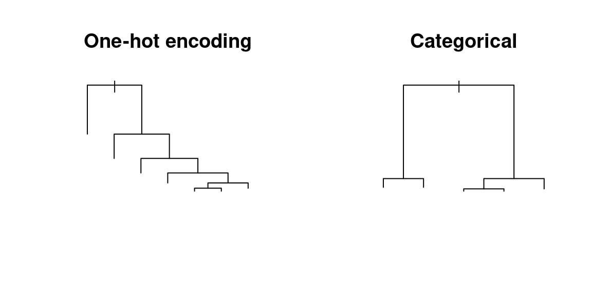
Notice the stark differences in tree structure between both options. On the left, the tree trained on the one-hot encoded data only shows growth on one side! This is the sparsity I was talking about before. On the right side, however, the tree based on the categorical variable shows a balanced and healthy structure. One-hot encoded data can easily mess up a single univariate regression tree, so imagine what it can do to your fancy random forest model with hundreds of these trees.
In the end, the magic of one-hot encoding is in its inherent ability to create two or three problems for each one it promised to solve. We all know someone like that. Not so hot, if you ask me.
Target Encoding, Mean Encoding, and Dummy Variables (All The Same)
On a bright summer day of 2001, Daniele Micci-Barreca finally got sick of the one-hot encoding wonders and decided to publish his ideas on a suitable alternative others later named mean encoding or target encoding. He told the story himself 20 years later, in a nice blog post titled Extending Target Encoding.
But what is target encoding? Let’s start with a continuous response variable y (a.k.a the target) and a categorical predictor x.
Mean Encoding
In it’s simplest form, target encoding replaces each category in x with the mean of y across the category cases. This results in a new numeric version of x named x_encoded in the example below.
yx |>
  dplyr::group_by(x) |>
  dplyr::mutate(
    x_encoded = mean(y)
  )
## # A tibble: 7 × 3
## # Groups:   x [3]
##       y x     x_encoded
##   <int> <chr>     <dbl>
## 1     1 a             2
## 2     2 a             2
## 3     3 a             2
## 4     4 b             5
## 5     5 b             5
## 6     6 b             5
## 7     7 c             7
Simple is good, right? But sometimes it’s not. In our toy case, the category “c” has only one case that maps directly to an actual value of y.Imagine the worst case scenario of x having one different category per row, then x_encoded would be identical to y!
Mean Encoding With Additive Smoothing
The issue can be solved by pushing the mean of y for each category in x towards the global mean of y by the weighted sample size of the category, as suggested by the expression
$$x\_encoded_i = \frac{n_i \times \overline{y}_i + m \times \overline{y}}{n_i + m}$$
where:
\(n_i\)is the size of the category\(i\).\(\overline{y}_i\)is the mean of the target over the category\(i\).\(m\)is the smoothing parameter.\(\overline{y}\)is the global mean of the target.
y_mean <- mean(yx$y)

m <- 3

yx |>
  dplyr::group_by(x) |>
  dplyr::mutate(
    x_encoded =
      (dplyr::n() * mean(y) + m * y_mean) / (dplyr::n() + m)
  )
## # A tibble: 7 × 3
## # Groups:   x [3]
##       y x     x_encoded
##   <int> <chr>     <dbl>
## 1     1 a          3
## 2     2 a          3
## 3     3 a          3
## 4     4 b          4.5
## 5     5 b          4.5
## 6     6 b          4.5
## 7     7 c          4.75
So far so good! But still, the simplest implementations of target encoding generate repeated values for all cases within a category. This can still mess-up tree-based models a bit, because splits may happen again and again in the same values of the predictor. However, there are several strategies to limit this issue as well.
Leave-one-out Target Encoding
In this version of target encoding, the encoded value of one case within a category is the mean of all other cases within the same category. This results in a robust encoding that avoids direct reference to the target value of the sample being encoded, and does not generate repeated values.
The code below implements the idea in a way so simple that it cannot even deal with one-case categories.
yx |>
  dplyr::group_by(x) |>
  dplyr::mutate(
    x_encoded = (sum(y) - y) / (dplyr::n() - 1)
  )
## # A tibble: 7 × 3
## # Groups:   x [3]
##       y x     x_encoded
##   <int> <chr>     <dbl>
## 1     1 a           2.5
## 2     2 a           2
## 3     3 a           1.5
## 4     4 b           5.5
## 5     5 b           5
## 6     6 b           4.5
## 7     7 c         NaN
Mean Encoding with White Noise
Another way to avoid repeated values while keeping the encoding as simple as possible consists of just adding a white noise to the encoded values. The code below adds noise generated by stats::runif() to the mean-encoded values, but other options such as stats::rnorm() (noise from a normal distribution) can be useful here. Since white noise is random, we need to set the seed of the pseudo-random number generator (with set.seed()) to obtain constant results every time we run the code below.
When using this method we have to be careful with the amount of noise we add. It should be a harmless fraction of target, small enough to not throw a model off the signal provided by the encoded variable. In our toy case y is between 1 and 7, so something like “one percent of the maximum” could work well here.
#maximum noise to add
max_noise <- max(yx$y)/100

#set seed for reproducibility
set.seed(1)

yx |>
  dplyr::group_by(x) |>
  dplyr::mutate(
    x_encoded = mean(y) + runif(n = dplyr::n(), max = max_noise)
  )
## # A tibble: 7 × 3
## # Groups:   x [3]
##       y x     x_encoded
##   <int> <chr>     <dbl>
## 1     1 a          2.02
## 2     2 a          2.03
## 3     3 a          2.04
## 4     4 b          5.06
## 5     5 b          5.01
## 6     6 b          5.06
## 7     7 c          7.07
This method can deal with one-case categories without issues, and does not generate repeated values, but in exchange, we have to be mindful of the amount of noise we add, and we have to set a random seed to ensure reproducibility.
Random Encoding
A more exotic non-deterministic method of encoding consists of computing the mean and the standard deviation of the target over the category, and then using these values to parameterize a normal distribution to extract randomized values from. This kind of encoding also requires to set the random seed to ensure reproducibility.
set.seed(1)

yx |>
  dplyr::group_by(x) |>
  dplyr::mutate(
    x_encoded = stats::rnorm(
      n = dplyr::n(),
      mean = mean(y),
      sd = ifelse(
        dplyr::n() == 1,
        stats::sd(yx$y), #use global sd for one-case groups
        stats::sd(y)     #use local sd for n-cases groups
      )
    )
  )
## # A tibble: 7 × 3
## # Groups:   x [3]
##       y x     x_encoded
##   <int> <chr>     <dbl>
## 1     1 a          1.37
## 2     2 a          2.18
## 3     3 a          1.16
## 4     4 b          6.60
## 5     5 b          5.33
## 6     6 b          4.18
## 7     7 c          8.05
Rank Encoding plus White Noise
This is a little different from all the other methods, because it does not map the categories to values from the target, but to the rank/order of the target means per category. It basically converts the categorical variable into an ordinal one arranged along with the target, and then adds white noise on top to avoid value repetition.
#maximum noise as function of the number of categories
max_noise <- length(unique(yx$x))/100

yx |>
  dplyr::arrange(y) |>
  dplyr::group_by(x) |>
  dplyr::mutate(
    x_encoded = dplyr::cur_group_id() + runif(n = dplyr::n(), max = max_noise)
  )
## # A tibble: 7 × 3
## # Groups:   x [3]
##       y x     x_encoded
##   <int> <chr>     <dbl>
## 1     1 a          1.02
## 2     2 a          1.01
## 3     3 a          1.02
## 4     4 b          2.03
## 5     5 b          2.01
## 6     6 b          2.02
## 7     7 c          3.03
The Target Encoding Lab
The function collinear::target_encoding_lab() implements all these encoding methods, and allows defining different combinations of parameters. It was designed to help understand how they work, and maybe help make choices about what’s the right encoding for a given categorical predictor.
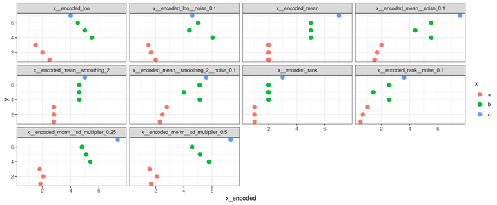
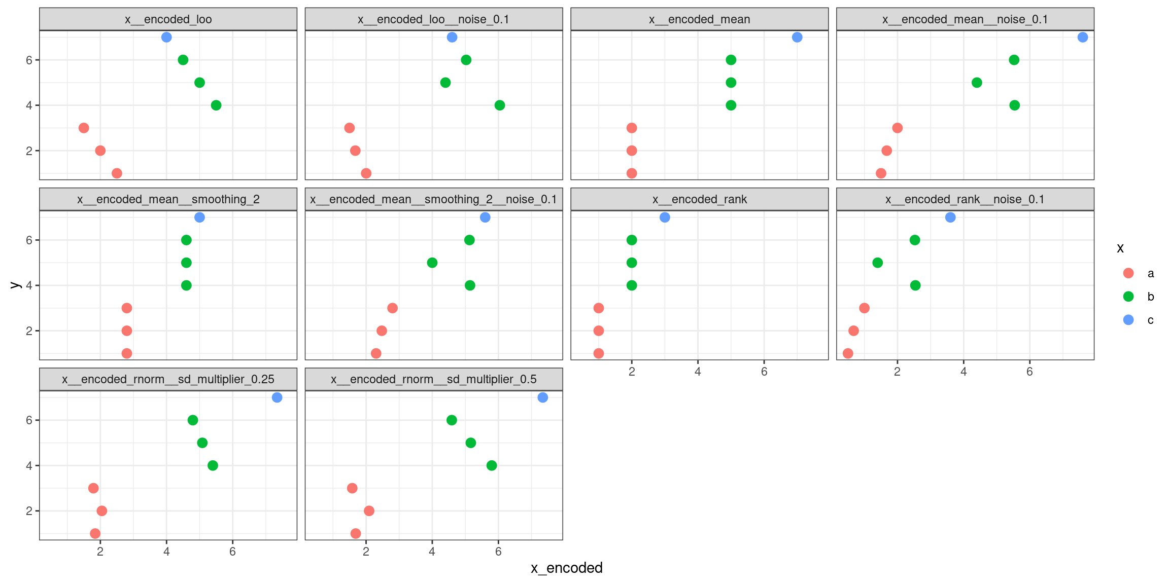
In the example below, the methods rank, mean, and leave-one-out are computed with white noise of 0 and 0.1 (that’s the width of the uniform distribution the noise is extracted from), the mean is also with and without smoothing, and the rnorm is computed using two different multipliers of the standard deviation of the normal distribution computed for each group in the predictor, just to help control the data spread.
The function also uses a random seed to generate the same noise across the encoded versions of the predictor to make them as comparable as possible. Every time you change the seed, results using white noise and the rnorm method should change as well.
yx_encoded <- target_encoding_lab(
  df = yx,
  response = "y",
  predictors = "x",
  white_noise = c(0, 0.1),
  smoothing = c(0, 2),
  rnorm_sd_multiplier = c(0.25, 0.5),
  verbose = TRUE,
  seed = 1, #for reproducibility
  replace = FALSE #to replace or not the predictors with their encodings
)
##
## Encoding the predictor: x
## New encoded predictor: 'x__encoded_rank'
## New encoded predictor: 'x__encoded_mean'
## New encoded predictor: 'x__encoded_mean__smoothing_2'
## New encoded predictor: 'x__encoded_loo'
## New encoded predictor: 'x__encoded_rank__noise_0.1'
## New encoded predictor: 'x__encoded_mean__noise_0.1'
## New encoded predictor: 'x__encoded_mean__smoothing_2__noise_0.1'
## New encoded predictor: 'x__encoded_loo__noise_0.1'
## New encoded predictor: 'x__encoded_rnorm__sd_multiplier_0.25'
## New encoded predictor: 'x__encoded_rnorm__sd_multiplier_0.5'
dplyr::glimpse(yx_encoded)
## Rows: 7
## Columns: 12
## $ y                                       <int> 1, 2, 3, 4, 5, 6, 7
## $ x                                       <chr> "a", "a", "a", "b", "b", "b", …
## $ x__encoded_rank                         <int> 1, 1, 1, 2, 2, 2, 3
## $ x__encoded_mean                         <dbl> 2, 2, 2, 5, 5, 5, 7
## $ x__encoded_mean__smoothing_2            <dbl> 2.8, 2.8, 2.8, 4.6, 4.6, 4.6, …
## $ x__encoded_loo                          <dbl> 2.5, 2.0, 1.5, 5.5, 5.0, 4.5, …
## $ x__encoded_rank__noise_0.1              <dbl> 0.5030858, 0.6752789, 0.999474…
## $ x__encoded_mean__noise_0.1              <dbl> 1.503086, 1.675279, 1.999475, …
## $ x__encoded_mean__smoothing_2__noise_0.1 <dbl> 2.303086, 2.475279, 2.799475, …
## $ x__encoded_loo__noise_0.1               <dbl> 2.003086, 1.675279, 1.499475, …
## $ x__encoded_rnorm__sd_multiplier_0.25    <dbl> 1.843387, 2.045911, 1.791093, …
## $ x__encoded_rnorm__sd_multiplier_0.5     <dbl> 1.686773, 2.091822, 1.582186, …
yx_encoded |>
  tidyr::pivot_longer(
    cols = dplyr::contains("__encoded"),
    values_to = "x_encoded"
  ) |>
  ggplot() +
  facet_wrap("name") +
  aes(
    x = x_encoded,
    y = y,
    color = x
  ) +
  geom_point(size = 3) +
  theme_bw()
 The function also allows to replace a given predictor with their selected encoding.
yx_encoded <- collinear::target_encoding_lab(
  df = yx,
  response = "y",
  predictors = "x",
  encoding_methods = "mean", #selected encoding method
  smoothing = 2,
  verbose = TRUE,
  replace = TRUE
)
## Warning in validate_df(df = df, min_rows = 30): the number of rows in 'df' is
## lower than 30. A multicollinearity analysis may fail or yield meaningless
## results.
dplyr::glimpse(yx_encoded)
## Rows: 7
## Columns: 2
## $ y <int> 1, 2, 3, 4, 5, 6, 7
## $ x <dbl> 2.8, 2.8, 2.8, 4.6, 4.6, 4.6, 5.0
And that’s all about target encoding so far!
I have a post in my TODO list with a little real experiment comparing target encoding with one-hot encoding in tree-based models. If you are interested, stay tuned!
Cheers,
Blas