Resources

• Rmarkdown notebook used in this tutorial
• Multicollinearity Hinders Model Interpretability
• R package collinear

Summary

In this detailed post, I dive deep into Variance Inflation Factors (VIF) and their crucial role in identifying multicollinearity within linear models. I use R code extensively to illustrate various concepts, making it a practical guide for those well-versed in R.

The post covers the following main points:

• VIF meaning and interpretation: Through practical examples, I demonstrate how to compute VIF values and their significance in model design. Particularly, I try to shed light on their influence on coefficient estimates and their confidence intervals.
• The Impact of High VIF: I use a small simulation to show how having a model design with a high VIF hinders the identification of predictors with moderate effects, particularly in situations with limited data.
• Effective VIF Management: I introduce how to use the collinear package and its vif_select() function. to aid in the selection of predictors with low VIF, thereby enhancing model stability and interpretability.

Ultimately, this post serves as a comprehensive resource for understanding, interpreting, and managing VIF in the context of linear modeling. It caters to those with a strong command of R and a keen interest in statistical modeling.

R packages

This tutorial requires the development version (>= 1.0.3) of the newly released R package collinear, and a few more.

#required
install.packages("remotes")
remotes::install_github(
  repo = "blasbenito/collinear", 
  ref = "development"
  )
install.packages("ranger")
install.packages("dplyr")
install.packages("ggplot2")

Example data

This post uses the toy data set shipped with the version >= 1.0.3 of the R package collinear. It is a data frame of centered and scaled variables representing a model design of the form y ~ a + b + c + d, where the predictors show varying degrees of relatedness. Let’s load and check it.

library(dplyr)
library(ggplot2)
library(collinear)

toy |> 
  round(3) |> 
  head()

##        y      a      b      c      d
## 1  0.655  0.342 -0.158  0.254  0.502
## 2  0.610  0.219  1.814  0.450  1.373
## 3  0.316  1.078 -0.643  0.580  0.673
## 4  0.202  0.956 -0.815  1.168 -0.147
## 5 -0.509 -0.149 -0.356 -0.456  0.187
## 6  0.675  0.465  1.292 -0.020  0.983

The columns in toy are related as follows:

• y: response generated from a and b using the expression y = a * 0.75 + b * 0.25 + noise.
• a: predictor of y uncorrelated with b.
• b: predictor of y uncorrelated with a.
• c: predictor generated as c = a + noise.
• d: predictor generated as d = (a + b)/2 + noise.

The pairwise correlations between all predictors in toy are shown below.

collinear::cor_df(
  df = toy,
  predictors = c("a", "b", "c", "d")
)

## # A tibble: 6 × 3
##   x     y     correlation
##   <chr> <chr>       <dbl>
## 1 c     a           0.962
## 2 d     b           0.639
## 3 d     a           0.636
## 4 d     c           0.615
## 5 b     a          -0.047
## 6 c     b          -0.042

Keep these pairwise correlations in mind for what comes next!

The Meaning of Variance Inflation Factors

There are two general cases of multicollinearity in model designs:

• When there are pairs of predictors highly correlated.
• When there are predictors that are linear combinations of other predictors.

The focus of this post is on the second one.

We can say a predictor is a linear combination of other predictors when it can be reasonably predicted from a multiple regression model against all other predictors.

Let’s say we focus on a and fit the multiple regression model a ~ b + c + d. The higher the R-squared of this model, the more confident we are to say that a is a linear combination of b + c + d.

#model of a against all other predictors
abcd_model <- lm(
  formula = a ~ b + c + d,
  data = toy
)

#r-squared of the a_model
abcd_R2 <- summary(abcd_model)$r.squared
abcd_R2

## [1] 0.9381214

Since the R-squared of a against all other predictors is pretty high, it definitely seems that a is a linear combination of the other predictors, and we can conclude that there is multicollinearity in the model design.

However, as informative as this R-squared is, it tells us nothing about the consequences of having multicollinearity in our model design. And this is where Variance Inflation Factors, or VIF for short, come into play.

What are Variance Inflation Factors?

The Variance Inflation Factor (VIF) of a predictor is computed as \(1/(1 - R^2)\), where \(R^²\) is the R-squared of the multiple linear regression of the predictor against all other predictors.

In the case of a, we just have to apply the VIF expression to the R-squared of the regression model against all other predictors.

abcd_vif <- 1/(1-abcd_R2)
abcd_vif

## [1] 16.16067

This VIF score is relative to the other predictors in the model design. If we change the model design, so does the VIF of all predictors! For example, if we remove c and d from the model design, we are left with this VIF for a:

ab_model <- lm(
  formula = a ~ b,
  data = toy
)

ab_vif <- 1/(1 - summary(ab_model)$r.squared)
ab_vif

## [1] 1.002253

An almost perfect VIF score!

We can simplify the VIF computation using collinear::vif_df(), which returns the VIF of a and b at once.

collinear::vif_df(
  df = toy[, c("a", "b")]
)

##   variable   vif
## 1        a 1.002
## 2        b 1.002

In plot below, the worst and best VIF scores of a are shown in the context of the relationship between R-squared and VIF, and three VIF thresholds commonly mentioned in the literature. These thresholds are represented as vertical dashed lines at VIF 2.5, 5, and 10, and are used as criteria to control multicollinearity in model designs. I will revisit this topic later in the post.

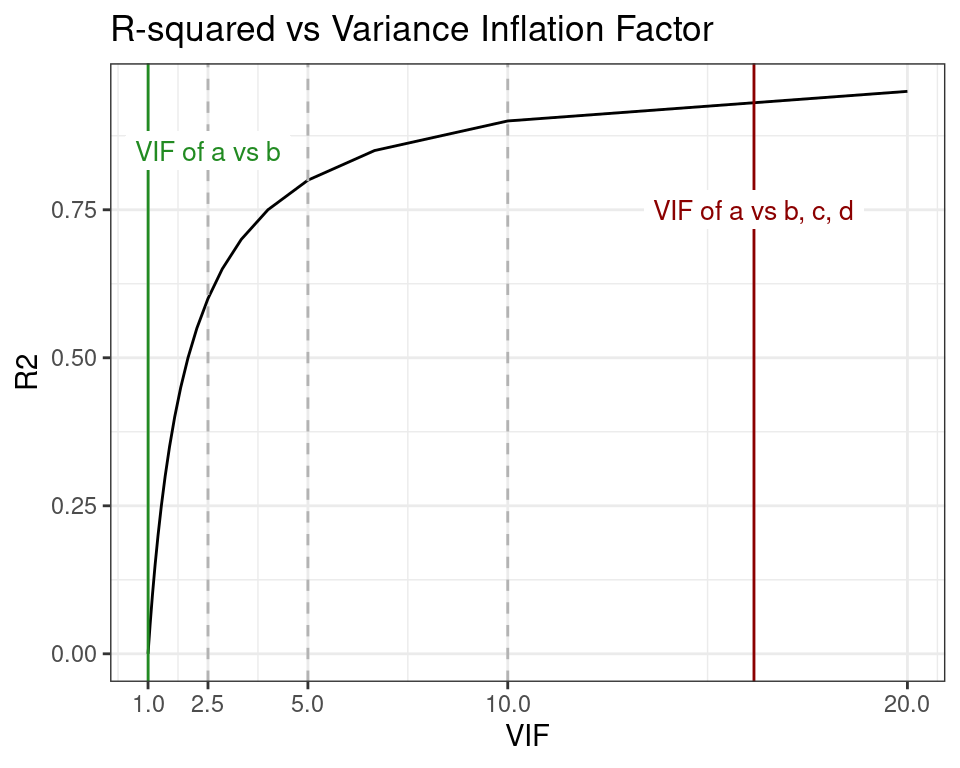
When the R-squared of the linear regression model is 0, then the VIF expression becomes \(1/(1 - 0) = 1\) and returns the minimum possible VIF. On the other end, when R-squared is 1, then we get \(1/(1 - 1) = Inf\), the maximum VIF.

So far, we have learned that to assess whether the predictor a induces multicollinearity in the model design y ~ a + b + c + d we can compute it’s Variance Inflation Factor from the R-squared of the model a ~ b + c + d. We have also learned that if the model design changes, so does the VIF of a. We also know that there are some magic numbers (the VIF thresholds) we can use as reference.

But still, we have no indication of what these VIF values actually mean! I will try to fix that in the next section.

But really, what are Variance Inflation Factors?

Variance Inflation Factors are inherently linked to these fundamental linear modeling concepts:

• Coefficient Estimate ($\hat{\beta}$): The estimated slope of the relationship between a predictor and the response in a linear model.
• Standard Error ($\text{SE}$): Represents the uncertainty around the estimation of the coefficient due to data variability.
• Significance level ($1.96$): The acceptable level of error when determining the significance of the coefficient estimate. Here it is simplified to 1.96, the 97.5th percentile of a normal distribution, to approximate a significance level of 0.05.
• Confidence Interval ($CI$): The range of values containing the true value of the coefficient estimate withing a certain significance level.

These terms are related by the expression to compute the confidence interval of the coefficient estimate:

$$\text{CI} = \beta \pm 1.96 \cdot \text{SE}$$ Let me convert this equation into a small function to compute confidence intervals of coefficient estimates named ci().

ci <- function(b, se){
  x <- se * 1.96
  as.numeric(c(b-x, b+x))
}
#note: stats::confint() which uses t-critical values to compute more precise confidence intervals. 

Now we are going to look at the coefficient estimate and standard error of a in the model y ~ a + b. We know that a in this model has a vif of 1.0022527.

yab_model <- lm(
  formula = y ~ a + b,
  data = toy
) |> 
  summary()

#coefficient estimate and standard error of a
a_coef <- yab_model$coefficients[2, 1:2]
a_coef

##    Estimate  Std. Error 
## 0.747689326 0.006636511

Now we plug them into our little function to compute the confidence interval.

a_ci <- ci(
  b = a_coef[1], 
  se = a_coef[2]
  )
a_ci

## [1] 0.7346818 0.7606969

And, finally, we compute the width of the confidence interval for a as the difference between the extremes of the confidence interval.

old_width <- diff(a_ci)
old_width

## [1] 0.02601512

Keep this number in mind, it’s important.

Now, let me tell you something weird: The confidence interval of a predictor is widened by a factor equal to the square root of its Variance Inflation Factor.

So, if the VIF of a predictor is, let’s say, 16, then this means that, in a linear model, multicollinearity is inflating the width of its confidence interval by a factor of 4.

In case you don’t want to take my word for it, here goes a demonstration. Now we fit the model y ~ a + b + c + d, where a has a vif of 16.1606674. If we follow the definition above, we could now expect an inflation of the confidence interval for a of about 4.0200333. Let’s find out if that’s the case!

#model y against all predictors and get summary
yabcd_model <- lm(
  formula = y ~ a + b + c + d,
  data = toy
) |> 
  summary()

#compute confidence interval of a
a_ci <- ci(
  b = yabcd_model$coefficients["a", "Estimate"], 
  se = yabcd_model$coefficients["a", "Std. Error"]
  )

#compute width of confidence interval of a
new_width <- diff(a_ci)
new_width

## [1] 0.1044793

Now, to find out the inflation factor of this new confidence interval, we divide it by the width of the old one.

new_width/old_width

## [1] 4.016101

And the result is VERY CLOSE to the square root of the VIF of a (4.0200333) in this model. Notice that this works because in the model y ~ a + b, a has a perfect VIF of 1.0022527. This demonstration needs a model with a quasi-perfect VIF as reference..

Now we can confirm our experiment about the meaning of VIF by repeating the exercise with b.

First we compute the VIF of b against a alone, and against a, c, and d, and the expected level of inflation of the confidence interval as the square root of the second VIF.

#vif of b vs a
ba_vif <- collinear::vif_df(
  df = toy[, c("a", "b")]
) |> 
  dplyr::filter(variable == "b")

#vif of b vs a c d
bacd_vif <- collinear::vif_df(
  df = toy[, c("a", "b", "c", "d")]
) |> 
  dplyr::filter(variable == "b")

#expeced inflation of the confidence interval
sqrt(bacd_vif$vif)

## [1] 2.01544

Now, since b is already in the models y ~ a + b and y ~ a + b + c + d, we just need to extract its coefficients, compute their confidence intervals, and divide one by the other to obtain the

#compute confidence interval of b in y ~ a + b
b_ci_old <- ci(
  b = yab_model$coefficients["b", "Estimate"], 
  se = yab_model$coefficients["b", "Std. Error"]
  )

#compute confidence interval of b in y ~ a + b + c + d
b_ci_new <- ci(
  b = yabcd_model$coefficients["b", "Estimate"], 
  se = yabcd_model$coefficients["b", "Std. Error"]
  )

#compute inflation
diff(b_ci_new)/diff(b_ci_old)

## [1] 2.013543

Again, the square root of the VIF of b in y ~ a + b + c + d is a great indicator of how much the confidence interval of b is inflated by multicollinearity in the model.

And that, folks, is the meaning of VIF.

When the VIF Hurts

In the previous sections we acquired an intuition of how Variance Inflation Factors measure the effect of multicollinearity in the precision of the coefficient estimates in a linear model. But there is more to that!

A coefficient estimate divided by its standard error results in the T statistic. This number is named “t value” in the table of coefficients shown below, and represents the distance (in number of standard errors) between the estimate and zero.

yabcd_model$coefficients[-1, ] |> 
  round(4)

##   Estimate Std. Error t value Pr(>|t|)
## a   0.7184     0.0267 26.9552   0.0000
## b   0.2596     0.0134 19.4253   0.0000
## c   0.0273     0.0232  1.1757   0.2398
## d   0.0039     0.0230  0.1693   0.8656

The p-value, named “Pr(>|t|)” above, is the probability of getting the T statistic when there is no effect of the predictor over the response. The part in italics is named the null hypothesis (H0), and happens when the confidence interval of the estimate intersects with zero, as in c and d.

ci(
  b = yabcd_model$coefficients["c", "Estimate"],
  se = yabcd_model$coefficients["c", "Std. Error"]
  )

## [1] -0.01819994  0.07276692

ci(
  b = yabcd_model$coefficients["d", "Estimate"],
  se = yabcd_model$coefficients["d", "Std. Error"]
  )

## [1] -0.04111146  0.04888457

The p-value of any predictor in the coefficients table above is computed as:

#predictor
predictor <- "d"

#number of cases
n <- nrow(toy)

#number of model terms
p <- nrow(yabcd_model$coefficients)

#one-tailed p-value
#q = absolute t-value
#df = degrees of freedom
p_value_one_tailed <- stats::pt(
  q = abs(yabcd_model$coefficients[predictor, "t value"]), 
  df = n - p #degrees of freedom
  )

#two-tailed p-value
2 * (1 - p_value_one_tailed)

## [1] 0.8655869

This p-value is then compared to a significance level (for example, 0.05 for a 95% confidence), which is just the lowest p-value acceptable as strong evidence to make a claim:

• p-value > significance: Evidence to claim that the predictor has no effect on the response. If the claim is wrong (we’ll see whey we could be wrong), we fall into a false negative (also Type II Error).
• p-value <= significance: Evidence to claim that the predictor has an effect on the response. If the claim is wrong, we fall into a false positive (also Type I Error).

Now, how does all this matter when talking about the Variance Inflation Factor? Because a high VIF triggers a cascade of effects that increases p-values that can mess up your claims about the importance of the predictors!

This cascade becomes a problem when the predictor has a small effect on the response, and the number of cases is small.

Let’s see how this works with b. This predictor has a solid effect on the response y (nonetheless, y was created as a * 0.75 + b * 0.25 + noise). It has a coefficient around 0.25, and a p-value of 0, so there is little to no risk of falling into a false negative when claiming that it is important to explain y, even when its confidence interval is inflated by a factor of two in the full model.

But let’s try a little experiment. We are going to create many small versions of toy, using only 30 cases selected by chance over a number of iterations, we are going to fit models in which b has a lower and a higher VIF, to monitor its p-values and estimates.

#number of repetitions
repetitions <- 1000

#number of cases to subset in toy
sample_size <- 30

#vectors to store results
lowvif_p_value <- 
  highvif_p_value <- 
  lowvif_estimate <-
  highvif_estimate <- 
  vector(length = repetitions)

#repetitions
for(i in 1:repetitions){
  
  #seed to make randomization reproducible
  set.seed(i)
  
  #toy subset
  toy.i <- toy[sample(x = 1:nrow(toy), size = sample_size), ]
  
  #high vif model
  highvif_model <- lm(
    formula =  y ~ a + b + c + d,
    data = toy.i
  ) |> 
    summary()
  
  #gather results of high vif model
  highvif_p_value[i] <- highvif_model$coefficients["b", "Pr(>|t|)"]
  highvif_estimate[i] <- highvif_model$coefficients["b", "Estimate"]
  
  #low_vif_model
  lowvif_model <- lm(
    formula =  y ~ a + b,
    data = toy.i
  ) |> 
    summary()
  
  #gather results of lowvif
  lowvif_p_value[i] <- lowvif_model$coefficients["b", "Pr(>|t|)"]
  lowvif_estimate[i] <- lowvif_model$coefficients["b", "Estimate"]
  
}

The plot below shows all p-values of the predictor b for the high and low VIF models across the experiment repetitions.

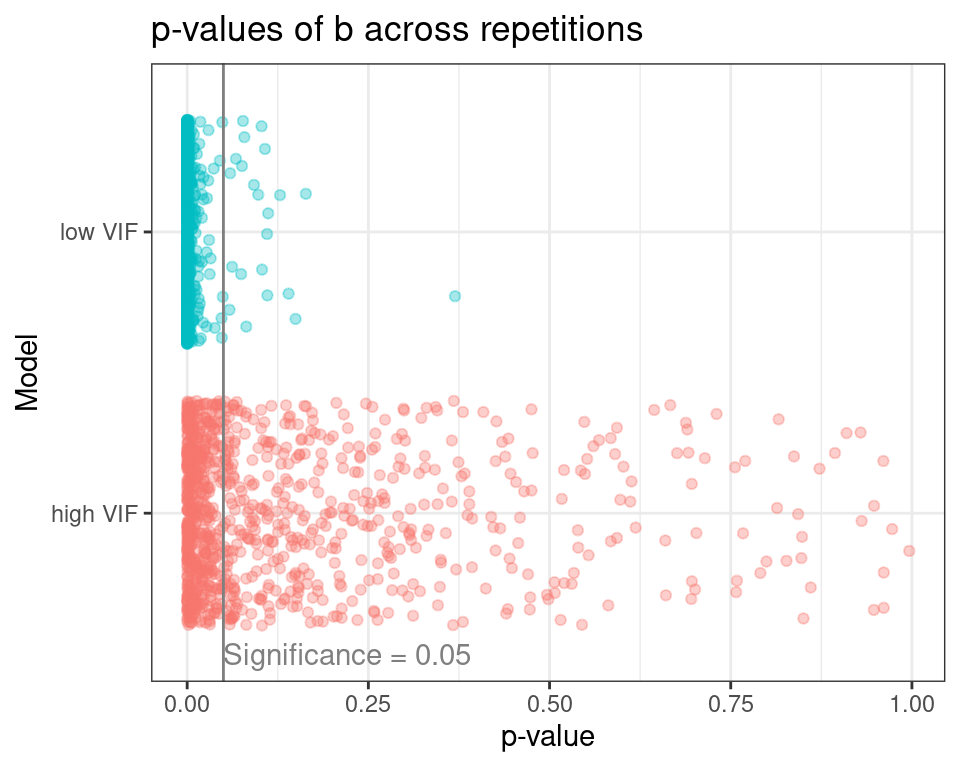
At a significance level of 0.05, the high VIF model rejects b as an important predictor of y on 53.5% of the model repetitions, while the low VIf model does the same on 2.2% of repetitions. This is a clear case of increase in Type II Error (false negatives) under multicollinearity.

Under multicollinearity, the probability of overlooking predictors with moderate effects increases dramatically!

The plot below shifts the focus towards the coefficient estimates for b across repetitions.

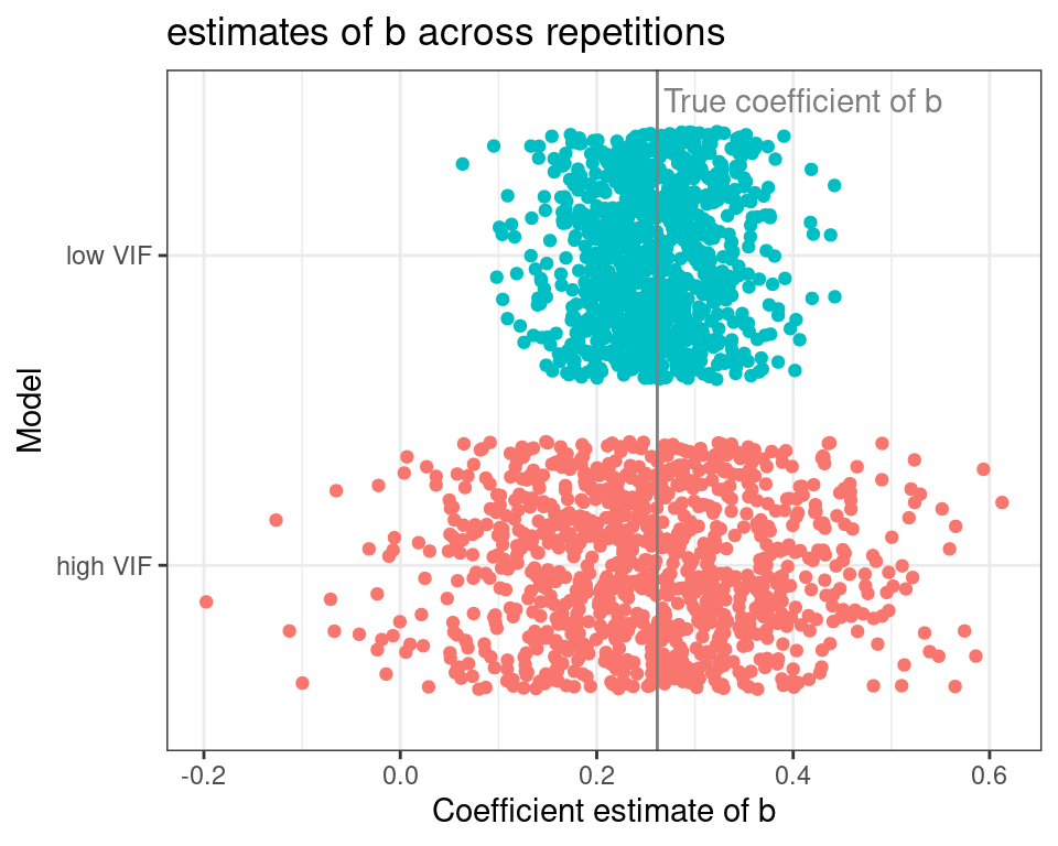
The gray vertical line represents the real value of the slope of b, and each dot represents a model repetition. The coefficients of the high VIF model are all over the place when compared to the low VIF one. Probably you have read somewhere that “multicollinearity induces model instability”, or something similar, and that is exactly what we are seeing here.

Finding the true effect of a predictor with a moderate effect becomes harder under multicollinearity.

Managing VIF in a Model Design

The second most common form of modeling self-sabotage is having high VIF predictors in a model design, just right after throwing deep learning at tabular problems to see what sticks. I don’t have solutions for the deep learning issue, but I have some pointers for the VIFs one: letting things go!. And with things I mean predictors, not the pictures of your old love. There is no rule the more predictors the better rule written anywhere relevant, and letting your model shed some fat is the best way to go here.

The collinear package has something to help here. The function collinear::vif_select() is specifically designed to help reduce VIF in a model design. And it can do it in two ways: either using domain knowledge to guide the process, or applying quantitative criteria instead.

Let’s follow the domain knowledge route first. Imagine you know a lot about y, you have read that a is very important to explain it, and you need to discuss this predictor in your results. But you are on the fence about the other predictors, so you don’t really care about what others are in the design. You can express such an idea using the argument preference_order, as shown below.

selected_predictors <- collinear::vif_select(
  df = toy,
  predictors = c("a", "b", "c", "d"),
  preference_order = "a",
  max_vif = 2.5
)
selected_predictors

## [1] "a" "b"

Now you have it, your new model design with a VIF below 2.5 is now y ~ a + b!

But what if you get new information and it turns out that d is also a variable of interest? Then you should just modify preference_order to include this new information.

selected_predictors <- collinear::vif_select(
  df = toy,
  predictors = c("a", "b", "c", "d"),
  preference_order = c("a", "d"),
  max_vif = 2.5
)
selected_predictors

## [1] "a" "d"

Notice that if your favorite variables are highly correlated, some of them are going to be removed anyway. For example, if a and c are your faves, since they are highly correlated, c is removed.

selected_predictors <- collinear::vif_select(
  df = toy,
  predictors = c("a", "b", "c", "d"),
  preference_order = c("a", "c"),
  max_vif = 2.5
)
selected_predictors

## [1] "a" "b"

In either case, you can now build your model while being sure that the coefficients of these predictors are going to be stable and precise.

Now, what if y is totally new for you, and you have no idea about what to use? In this case, the function collinear::preference_order() helps you rank the predictors following a quantiative criteria, and after that, collinear::vif_select() can use it to reduce your VIFs.

By default, collinear::preference_order() calls collinear::f_rsquared() to compute the R-squared between each predictor and the response variable (that’s why the argument response is required here), to return a data frame with the variables ranked from “better” to “worse”.

preference <- collinear::preference_order(
  df = toy,
  response = "y",
  predictors = c("a", "b", "c", "d"),
  f = f_rsquared
)

preference

##   predictor preference
## 1         a 0.77600503
## 2         c 0.72364944
## 3         d 0.59345954
## 4         b 0.07343563

Now you can use this data frame as input for the argument preference_order:

selected_predictors <- collinear::vif_select(
  df = toy,
  predictors = c("a", "b", "c", "d"),
  preference_order = preference,
  max_vif = 2.5
)
selected_predictors

## [1] "a" "d"

Now at least you can be sure that the predictors in your model design have low VIF, and were selected taking their correlation with the response as criteria.

Well, I think that’s enough for today. I hope you found this post helpful. Have a great time!

Blas