R package collinear

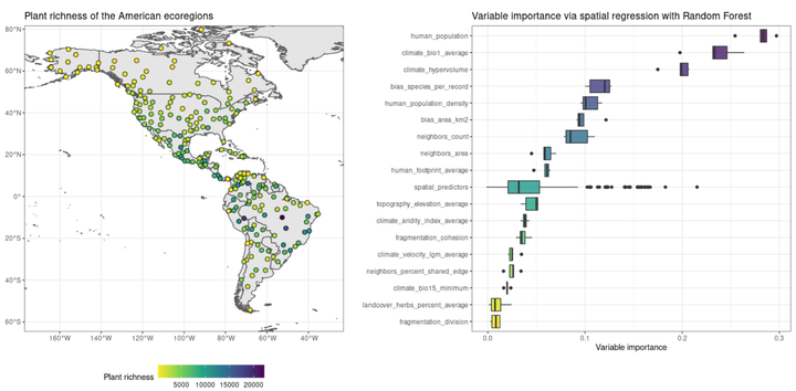
Graph by Blas M. Benito

DOI CRAN status CRAN\_Download\_Badge R-CMD-check

Summary

The R package collinear combines four different methods to offer a comprehensive tool for multicollinearity management:

  • Pairwise correlation for numeric and categorical predictors: computed either via Pearson or Spearman methods for numeric predictors, and Cramer’s V for categorical predictors.
  • Variance Inflation Factor analysis (VIF): to identify multicollinearity resulting from predictors being linear combinations of other predictors.
  • Target encoding of categorical predictors: to convert them to numeric using a numeric variable as response (usually a response variable) and handle them as numerics during the multicollinearity filtering.
  • Variable prioritization: method to prioritize predictors during variable selection either using expert knowledge or quantitative criteria.

These methods are integrated in the collinear() function, which returns a vector of selected predictors with a controlled multicollinearity.

selected_variables <- collinear(
  df, #your data frame
  response, #name of your response variable
  predictors, #names of your predictors,
  preference_order, #your predictors in order of interest
  max_cor, #maximum bivariate correlation
  max_vif, #maximum variance inflation factor
  encoding_method, #method to convert categorical predictors into numerics
)

The package contains other functions that may be useful during multicollinearity management:

  • cor_select(): like collinear(), but only using pairwise correlations.
  • vif_select(): like collinear(), but only using variance inflation factors.
  • preference_order(): to compute preference order based on univariate models.
  • target_encoding_lab(): to convert categorical predictors into numeric using several methods.
  • cor_df(): to generate a data frame with all pairwise correlation scores.
  • cor_matrix(): to convert a correlation data frame into matrix, or obtain a correlation matrix.
  • vif_df(): to obtain a data frame with all variance inflation factors.

Citation

If you found this package useful during your research work, please cite it as:

Blas M. Benito (2023). collinear: R Package for Seamless Multicollinearity Management. Version 1.0.1. doi: 10.5281/zenodo.10039489

Install

The package collinear can be installed from CRAN.

install.packages("collinear")
library(collinear)

The development version can be installed from GitHub.

remotes::install_github(
  repo = "blasbenito/collinear", 
  ref = "development"
  )

Multicollinearity management with the collinear package.

This section shows the basic usage of the package and offers a brief explanation on the methods used within.

Required libraries and example data

The libraries below are required to run the examples in this section.

library(collinear)
library(dplyr)
library(tictoc)

The package collinear is shipped with a data frame named vi, with 30.000 rows and 67 columns with a mixture of numeric and categorical variables.

dplyr::glimpse(vi)
## Rows: 30,000
## Columns: 67
## $ longitude                  <dbl> -114.254306, 114.845693, -122.145972, 108.3…
## $ latitude                   <dbl> 45.0540272, 26.2706940, 56.3790272, 29.9456…
## $ vi_mean                    <dbl> 0.38, 0.53, 0.45, 0.69, 0.42, 0.68, 0.70, 0…
## $ vi_max                     <dbl> 0.57, 0.67, 0.65, 0.85, 0.64, 0.78, 0.77, 0…
## $ vi_min                     <dbl> 0.12, 0.41, 0.25, 0.50, 0.25, 0.48, 0.60, 0…
## $ vi_range                   <dbl> 0.45, 0.26, 0.40, 0.34, 0.39, 0.31, 0.17, 0…
## $ koppen_zone                <chr> "BSk", "Cfa", "Dfc", "Cfb", "Aw", "Cfa", "A…
## $ koppen_group               <chr> "Arid", "Temperate", "Cold", "Temperate", "…
## $ koppen_description         <chr> "steppe, cold", "no dry season, hot summer"…
## $ soil_type                  <chr> "Cambisols", "Acrisols", "Luvisols", "Aliso…
## $ topo_slope                 <int> 6, 2, 0, 10, 0, 10, 6, 0, 2, 0, 0, 1, 0, 1,…
## $ topo_diversity             <int> 29, 24, 21, 25, 19, 30, 26, 20, 26, 22, 25,…
## $ topo_elevation             <int> 1821, 143, 765, 1474, 378, 485, 604, 1159, …
## $ swi_mean                   <dbl> 27.5, 56.1, 41.4, 59.3, 37.4, 56.3, 52.3, 2…
## $ swi_max                    <dbl> 62.9, 74.4, 81.9, 81.1, 83.2, 73.8, 55.8, 3…
## $ swi_min                    <dbl> 24.5, 33.3, 42.2, 31.3, 8.3, 28.8, 25.3, 11…
## $ swi_range                  <dbl> 38.4, 41.2, 39.7, 49.8, 74.9, 45.0, 30.5, 2…
## $ soil_temperature_mean      <dbl> 4.8, 19.9, 1.2, 13.0, 28.2, 18.1, 21.5, 23.…
## $ soil_temperature_max       <dbl> 29.9, 32.6, 20.4, 24.6, 41.6, 29.1, 26.4, 4…
## $ soil_temperature_min       <dbl> -12.4, 3.9, -16.0, -0.4, 16.8, 4.1, 17.3, 5…
## $ soil_temperature_range     <dbl> 42.3, 28.8, 36.4, 25.0, 24.8, 24.9, 9.1, 38…
## $ soil_sand                  <int> 41, 39, 27, 29, 48, 33, 30, 78, 23, 64, 54,…
## $ soil_clay                  <int> 20, 24, 28, 31, 27, 29, 40, 15, 26, 22, 23,…
## $ soil_silt                  <int> 38, 35, 43, 38, 23, 36, 29, 6, 49, 13, 22, …
## $ soil_ph                    <dbl> 6.5, 5.9, 5.6, 5.5, 6.5, 5.8, 5.2, 7.1, 7.3…
## $ soil_soc                   <dbl> 43.1, 14.6, 36.4, 34.9, 8.1, 20.8, 44.5, 4.…
## $ soil_nitrogen              <dbl> 2.8, 1.3, 2.9, 3.6, 1.2, 1.9, 2.8, 0.6, 3.1…
## $ solar_rad_mean             <dbl> 17.634, 19.198, 13.257, 14.163, 24.512, 17.…
## $ solar_rad_max              <dbl> 31.317, 24.498, 25.283, 17.237, 28.038, 22.…
## $ solar_rad_min              <dbl> 5.209, 13.311, 1.587, 9.642, 19.102, 12.196…
## $ solar_rad_range            <dbl> 26.108, 11.187, 23.696, 7.595, 8.936, 10.20…
## $ growing_season_length      <dbl> 139, 365, 164, 333, 228, 365, 365, 60, 365,…
## $ growing_season_temperature <dbl> 12.65, 19.35, 11.55, 12.45, 26.45, 17.75, 2…
## $ growing_season_rainfall    <dbl> 224.5, 1493.4, 345.4, 1765.5, 984.4, 1860.5…
## $ growing_degree_days        <dbl> 2140.5, 7080.9, 2053.2, 4162.9, 10036.7, 64…
## $ temperature_mean           <dbl> 3.65, 19.35, 1.45, 11.35, 27.55, 17.65, 22.…
## $ temperature_max            <dbl> 24.65, 33.35, 21.15, 23.75, 38.35, 30.55, 2…
## $ temperature_min            <dbl> -14.05, 3.05, -18.25, -3.55, 19.15, 2.45, 1…
## $ temperature_range          <dbl> 38.7, 30.3, 39.4, 27.3, 19.2, 28.1, 7.0, 29…
## $ temperature_seasonality    <dbl> 882.6, 786.6, 1070.9, 724.7, 219.3, 747.2, …
## $ rainfall_mean              <int> 446, 1493, 560, 1794, 990, 1860, 3150, 356,…
## $ rainfall_min               <int> 25, 37, 24, 29, 0, 60, 122, 1, 10, 12, 0, 0…
## $ rainfall_max               <int> 62, 209, 87, 293, 226, 275, 425, 62, 256, 3…
## $ rainfall_range             <int> 37, 172, 63, 264, 226, 215, 303, 61, 245, 2…
## $ evapotranspiration_mean    <dbl> 78.32, 105.88, 50.03, 64.65, 156.60, 108.50…
## $ evapotranspiration_max     <dbl> 164.70, 190.86, 117.53, 115.79, 187.71, 191…
## $ evapotranspiration_min     <dbl> 13.67, 50.44, 3.53, 28.01, 128.59, 51.39, 8…
## $ evapotranspiration_range   <dbl> 151.03, 140.42, 113.99, 87.79, 59.13, 139.9…
## $ cloud_cover_mean           <int> 31, 48, 42, 64, 38, 52, 60, 13, 53, 20, 11,…
## $ cloud_cover_max            <int> 39, 61, 49, 71, 58, 67, 77, 18, 60, 27, 23,…
## $ cloud_cover_min            <int> 16, 34, 33, 54, 19, 39, 45, 6, 45, 14, 2, 1…
## $ cloud_cover_range          <int> 23, 27, 15, 17, 38, 27, 32, 11, 15, 12, 21,…
## $ aridity_index              <dbl> 0.54, 1.27, 0.90, 2.08, 0.55, 1.67, 2.88, 0…
## $ humidity_mean              <dbl> 55.56, 62.14, 59.87, 69.32, 51.60, 62.76, 7…
## $ humidity_max               <dbl> 63.98, 65.00, 68.19, 71.90, 67.07, 65.68, 7…
## $ humidity_min               <dbl> 48.41, 58.97, 53.75, 67.21, 33.89, 59.92, 7…
## $ humidity_range             <dbl> 15.57, 6.03, 14.44, 4.69, 33.18, 5.76, 3.99…
## $ biogeo_ecoregion           <chr> "South Central Rockies forests", "Jian Nan …
## $ biogeo_biome               <chr> "Temperate Conifer Forests", "Tropical & Su…
## $ biogeo_realm               <chr> "Nearctic", "Indomalayan", "Nearctic", "Pal…
## $ country_name               <chr> "United States of America", "China", "Canad…
## $ country_population         <dbl> 313973000, 1338612970, 33487208, 1338612970…
## $ country_gdp                <dbl> 15094000, 7973000, 1300000, 7973000, 15860,…
## $ country_income             <chr> "1. High income: OECD", "3. Upper middle in…
## $ continent                  <chr> "North America", "Asia", "North America", "…
## $ region                     <chr> "Americas", "Asia", "Americas", "Asia", "Af…
## $ subregion                  <chr> "Northern America", "Eastern Asia", "Northe…

The response variables are “vi_mean”, “vi_max”, “vi_min”, and “vi_range”, with statistics of a vegetation index named NDVI. The predictors are stored in the character vector vi_predictors.

vi_predictors
##  [1] "koppen_zone"                "koppen_group"              
##  [3] "koppen_description"         "soil_type"                 
##  [5] "topo_slope"                 "topo_diversity"            
##  [7] "topo_elevation"             "swi_mean"                  
##  [9] "swi_max"                    "swi_min"                   
## [11] "swi_range"                  "soil_temperature_mean"     
## [13] "soil_temperature_max"       "soil_temperature_min"      
## [15] "soil_temperature_range"     "soil_sand"                 
## [17] "soil_clay"                  "soil_silt"                 
## [19] "soil_ph"                    "soil_soc"                  
## [21] "soil_nitrogen"              "solar_rad_mean"            
## [23] "solar_rad_max"              "solar_rad_min"             
## [25] "solar_rad_range"            "growing_season_length"     
## [27] "growing_season_temperature" "growing_season_rainfall"   
## [29] "growing_degree_days"        "temperature_mean"          
## [31] "temperature_max"            "temperature_min"           
## [33] "temperature_range"          "temperature_seasonality"   
## [35] "rainfall_mean"              "rainfall_min"              
## [37] "rainfall_max"               "rainfall_range"            
## [39] "evapotranspiration_mean"    "evapotranspiration_max"    
## [41] "evapotranspiration_min"     "evapotranspiration_range"  
## [43] "cloud_cover_mean"           "cloud_cover_max"           
## [45] "cloud_cover_min"            "cloud_cover_range"         
## [47] "aridity_index"              "humidity_mean"             
## [49] "humidity_max"               "humidity_min"              
## [51] "humidity_range"             "biogeo_ecoregion"          
## [53] "biogeo_biome"               "biogeo_realm"              
## [55] "country_name"               "country_population"        
## [57] "country_gdp"                "country_income"            
## [59] "continent"                  "region"                    
## [61] "subregion"

collinear()

The collinear() function applies a multicollinearity filtering to numeric and categorical variables via pairwise correlations (with cor_select()) and variance inflation factors (with vif_select()). Categorical variables are converted into numeric via target-encoding (with target_encoding_lab()) using a response variable as reference. If the response variable is not provided, categorical variables are ignored.

Input arguments

The function takes these inputs:

  • df: a data frame with predictors, and preferably, a response (more about this later).
  • response: the name of the response variable, only relevant and highly recommended if there are categorical variables within the predictors.
  • predictors: names of predictors involved in the multicollinearity analysis.
  • preference_order: names of the predictors in the user’s order of preference. Does not need to name all predictors in predictors!
  • cor_method: usually “pearson”, but also “spearman” is accepted.
  • max_cor: maximum correlation allowed between two predictors.
  • max_vif: maximum VIF allowed in a predictor.
  • encoding_method: method used to convert categorical variables into numeric. Only relevant when a response is provided. By default, each group of the categorical variable is encoded with the mean of the response across the group.

The code below shows a quick example. Notice that the argument preference_order was left as NULL, but will be explained later.

selected_predictors <- collinear(
  df = vi,
  response = "vi_mean",
  predictors = vi_predictors,
  preference_order = NULL,
  max_cor = 0.75,
  max_vif = 5,
  encoding_method = "mean"
)

selected_predictors
##  [1] "country_income"             "topo_diversity"            
##  [3] "topo_slope"                 "country_population"        
##  [5] "country_gdp"                "humidity_range"            
##  [7] "soil_soc"                   "region"                    
##  [9] "soil_clay"                  "soil_type"                 
## [11] "subregion"                  "biogeo_realm"              
## [13] "soil_sand"                  "topo_elevation"            
## [15] "soil_nitrogen"              "swi_range"                 
## [17] "koppen_group"               "swi_min"                   
## [19] "solar_rad_max"              "rainfall_min"              
## [21] "growing_season_temperature" "rainfall_range"            
## [23] "solar_rad_min"              "cloud_cover_range"

The function has returned a list of predictors that should have a correlation lower than 0.75 with each other, and a VIF lower than 5. Let’s see if that’s true.

The function cor_df() returns a data frame with pairwise correlations, arranged by the absolute value of the correlation.

selected_predictors_cor <- cor_df(
  df = vi,
  response = "vi_mean",
  predictors = selected_predictors
)
head(selected_predictors_cor)
## # A tibble: 6 × 3
##   x             y                          correlation
##   <chr>         <chr>                            <dbl>
## 1 solar_rad_min growing_season_temperature       0.744
## 2 koppen_group  soil_type                        0.732
## 3 soil_nitrogen soil_soc                         0.729
## 4 swi_min       soil_nitrogen                    0.673
## 5 soil_sand     soil_clay                       -0.666
## 6 koppen_group  swi_range                        0.659

The data frame above shows that the maximum correlation between two of the selected predictors is below 0.75, so here collinear() worked as expected.

The function vif_df() returns a data frame with the VIF scores of all predictors.

selected_predictors_vif <- vif_df(
  df = vi,
  response = "vi_mean",
  predictors = selected_predictors
)
selected_predictors_vif
##                      variable   vif
## 1              country_income 1.215
## 2              topo_diversity 1.662
## 3                  topo_slope 1.929
## 4              humidity_range 2.043
## 5              topo_elevation 2.101
## 6                 country_gdp 2.158
## 7          country_population 2.171
## 8                rainfall_min 2.269
## 9           cloud_cover_range 2.418
## 10                   soil_soc 2.744
## 11                     region 2.849
## 12             rainfall_range 2.876
## 13                  subregion 2.900
## 14                  soil_clay 2.966
## 15                  soil_type 2.991
## 16              solar_rad_max 3.145
## 17               biogeo_realm 3.150
## 18                  soil_sand 3.175
## 19              soil_nitrogen 3.376
## 20                    swi_min 3.450
## 21                  swi_range 3.781
## 22               koppen_group 4.151
## 23 growing_season_temperature 4.314
## 24              solar_rad_min 4.432

The output shows that the maximum VIF is 4.2, so here collinear() did its work as expected.

Arguments max_cor and max_vif

The arguments max_cor and max_vif control the intensity of the multicollinearity filtering.

#restrictive setup
selected_predictors_restrictive <- collinear(
  df = vi,
  response = "vi_mean",
  predictors = vi_predictors,
  max_cor = 0.5,
  max_vif = 2.5
)

#permissive setup
selected_predictors_permissive <- collinear(
  df = vi,
  response = "vi_mean",
  predictors = vi_predictors,
  max_cor = 0.9,
  max_vif = 10
)

These are the variables selected under a restrictive setup:

selected_predictors_restrictive
##  [1] "country_income"             "soil_clay"                 
##  [3] "country_population"         "topo_slope"                
##  [5] "humidity_range"             "topo_elevation"            
##  [7] "soil_soc"                   "soil_silt"                 
##  [9] "cloud_cover_range"          "region"                    
## [11] "solar_rad_max"              "growing_season_temperature"
## [13] "biogeo_realm"

These are the variables selected under a more permissive setup:

selected_predictors_permissive
##  [1] "country_income"             "topo_diversity"            
##  [3] "topo_slope"                 "country_population"        
##  [5] "country_gdp"                "soil_soc"                  
##  [7] "region"                     "soil_type"                 
##  [9] "soil_nitrogen"              "subregion"                 
## [11] "biogeo_realm"               "topo_elevation"            
## [13] "koppen_group"               "biogeo_biome"              
## [15] "country_name"               "soil_ph"                   
## [17] "aridity_index"              "growing_season_temperature"
## [19] "rainfall_min"               "rainfall_range"            
## [21] "swi_mean"                   "soil_temperature_max"      
## [23] "solar_rad_mean"             "temperature_seasonality"   
## [25] "soil_clay"                  "soil_silt"                 
## [27] "cloud_cover_min"            "swi_range"                 
## [29] "humidity_range"

As expected, the restrictive setup resulted in a smaller set of selected predictors. There are no hard rules for max_cor and max_vif, and their selection will depend on the objective of the analysis and the nature of the predictors.

The response argument

The response argument is used to encode categorical variables as numeric. When omitted, the collinear() function ignores categorical variables. However, the function cor_select() can help when there is not a suitable response variable in a data frame. This option is discussed at the end of this section.

selected_predictors_response <- collinear(
  df = vi,
  response = "vi_mean",
  predictors = vi_predictors
)

selected_predictors_no_response <- collinear(
  df = vi,
  predictors = vi_predictors
)

When the argument response is used, the output may contain categorical predictors (tagged with <chr>, from “character” below).

dplyr::glimpse(vi[, selected_predictors_response])
## Rows: 30,000
## Columns: 24
## $ country_income             <chr> "1. High income: OECD", "3. Upper middle in…
## $ topo_diversity             <int> 29, 24, 21, 25, 19, 30, 26, 20, 26, 22, 25,…
## $ topo_slope                 <int> 6, 2, 0, 10, 0, 10, 6, 0, 2, 0, 0, 1, 0, 1,…
## $ country_population         <dbl> 313973000, 1338612970, 33487208, 1338612970…
## $ country_gdp                <dbl> 15094000, 7973000, 1300000, 7973000, 15860,…
## $ humidity_range             <dbl> 15.57, 6.03, 14.44, 4.69, 33.18, 5.76, 3.99…
## $ soil_soc                   <dbl> 43.1, 14.6, 36.4, 34.9, 8.1, 20.8, 44.5, 4.…
## $ region                     <chr> "Americas", "Asia", "Americas", "Asia", "Af…
## $ soil_clay                  <int> 20, 24, 28, 31, 27, 29, 40, 15, 26, 22, 23,…
## $ soil_type                  <chr> "Cambisols", "Acrisols", "Luvisols", "Aliso…
## $ subregion                  <chr> "Northern America", "Eastern Asia", "Northe…
## $ biogeo_realm               <chr> "Nearctic", "Indomalayan", "Nearctic", "Pal…
## $ soil_sand                  <int> 41, 39, 27, 29, 48, 33, 30, 78, 23, 64, 54,…
## $ topo_elevation             <int> 1821, 143, 765, 1474, 378, 485, 604, 1159, …
## $ soil_nitrogen              <dbl> 2.8, 1.3, 2.9, 3.6, 1.2, 1.9, 2.8, 0.6, 3.1…
## $ swi_range                  <dbl> 38.4, 41.2, 39.7, 49.8, 74.9, 45.0, 30.5, 2…
## $ koppen_group               <chr> "Arid", "Temperate", "Cold", "Temperate", "…
## $ swi_min                    <dbl> 24.5, 33.3, 42.2, 31.3, 8.3, 28.8, 25.3, 11…
## $ solar_rad_max              <dbl> 31.317, 24.498, 25.283, 17.237, 28.038, 22.…
## $ rainfall_min               <int> 25, 37, 24, 29, 0, 60, 122, 1, 10, 12, 0, 0…
## $ growing_season_temperature <dbl> 12.65, 19.35, 11.55, 12.45, 26.45, 17.75, 2…
## $ rainfall_range             <int> 37, 172, 63, 264, 226, 215, 303, 61, 245, 2…
## $ solar_rad_min              <dbl> 5.209, 13.311, 1.587, 9.642, 19.102, 12.196…
## $ cloud_cover_range          <int> 23, 27, 15, 17, 38, 27, 32, 11, 15, 12, 21,…

However, when the argument response is ignored, all categorical predictors are ignored.

dplyr::glimpse(vi[, selected_predictors_no_response])
## Rows: 30,000
## Columns: 18
## $ topo_diversity             <int> 29, 24, 21, 25, 19, 30, 26, 20, 26, 22, 25,…
## $ country_gdp                <dbl> 15094000, 7973000, 1300000, 7973000, 15860,…
## $ country_population         <dbl> 313973000, 1338612970, 33487208, 1338612970…
## $ topo_slope                 <int> 6, 2, 0, 10, 0, 10, 6, 0, 2, 0, 0, 1, 0, 1,…
## $ soil_soc                   <dbl> 43.1, 14.6, 36.4, 34.9, 8.1, 20.8, 44.5, 4.…
## $ soil_clay                  <int> 20, 24, 28, 31, 27, 29, 40, 15, 26, 22, 23,…
## $ soil_sand                  <int> 41, 39, 27, 29, 48, 33, 30, 78, 23, 64, 54,…
## $ soil_nitrogen              <dbl> 2.8, 1.3, 2.9, 3.6, 1.2, 1.9, 2.8, 0.6, 3.1…
## $ humidity_range             <dbl> 15.57, 6.03, 14.44, 4.69, 33.18, 5.76, 3.99…
## $ topo_elevation             <int> 1821, 143, 765, 1474, 378, 485, 604, 1159, …
## $ cloud_cover_range          <int> 23, 27, 15, 17, 38, 27, 32, 11, 15, 12, 21,…
## $ solar_rad_max              <dbl> 31.317, 24.498, 25.283, 17.237, 28.038, 22.…
## $ rainfall_min               <int> 25, 37, 24, 29, 0, 60, 122, 1, 10, 12, 0, 0…
## $ growing_season_temperature <dbl> 12.65, 19.35, 11.55, 12.45, 26.45, 17.75, 2…
## $ rainfall_range             <int> 37, 172, 63, 264, 226, 215, 303, 61, 245, 2…
## $ swi_range                  <dbl> 38.4, 41.2, 39.7, 49.8, 74.9, 45.0, 30.5, 2…
## $ solar_rad_min              <dbl> 5.209, 13.311, 1.587, 9.642, 19.102, 12.196…
## $ swi_min                    <dbl> 24.5, 33.3, 42.2, 31.3, 8.3, 28.8, 25.3, 11…

If there are categorical variables in a data frame, but there is no suitable response variable, then the function cor_select() can handle the multicollinearity management via pairwise correlations, but at a MUCH higher computational cost, and with different results, as shown below.

tictoc::tic()
selected_predictors_response <- cor_select(
  df = vi,
  response = "vi_mean",
  predictors = vi_predictors
)
tictoc::toc()
## 0.429 sec elapsed
tictoc::tic()
selected_predictors_no_response <- cor_select(
  df = vi,
  predictors = vi_predictors
)
tictoc::toc()
## 34.945 sec elapsed
selected_predictors_response
##  [1] "country_population"         "topo_elevation"            
##  [3] "country_income"             "country_gdp"               
##  [5] "topo_slope"                 "humidity_range"            
##  [7] "soil_clay"                  "topo_diversity"            
##  [9] "soil_sand"                  "cloud_cover_range"         
## [11] "region"                     "growing_season_temperature"
## [13] "solar_rad_min"              "soil_soc"                  
## [15] "rainfall_min"               "swi_range"                 
## [17] "soil_nitrogen"              "rainfall_range"            
## [19] "temperature_max"            "swi_min"                   
## [21] "subregion"                  "temperature_seasonality"   
## [23] "biogeo_realm"               "cloud_cover_min"           
## [25] "soil_type"                  "aridity_index"             
## [27] "solar_rad_max"              "koppen_group"              
## [29] "cloud_cover_max"
selected_predictors_no_response
##  [1] "topo_elevation"             "topo_slope"                
##  [3] "country_population"         "topo_diversity"            
##  [5] "soil_clay"                  "humidity_range"            
##  [7] "soil_sand"                  "country_gdp"               
##  [9] "cloud_cover_range"          "country_income"            
## [11] "rainfall_min"               "soil_soc"                  
## [13] "swi_range"                  "growing_season_temperature"
## [15] "rainfall_range"             "soil_nitrogen"             
## [17] "solar_rad_min"              "aridity_index"             
## [19] "cloud_cover_min"            "temperature_max"           
## [21] "region"                     "swi_min"                   
## [23] "solar_rad_max"              "evapotranspiration_range"  
## [25] "swi_mean"                   "humidity_max"              
## [27] "soil_type"

The variable selection results differ because the numeric representations of the categorical variables are rather different between the two options. When no response is provided, the function cor_select() compares categorical predictors against numeric ones by encoding each categorical after each numeric, and compares pairs of categoricals using Cramer’s V, implemented in the function cramer_v(). Additionally, Cramer’s V values are not directly comparable with Pearson or Spearman correlation scores, and having them together in the same analysis might induce bias during the variable selection. Not using the response argument should always be the last option.

Preference order

The argument preference_order gives the user some control on what predictors should be removed first and what predictors should be kept during the multicollinearity filtering. This argument accepts a vector of predictor names in the order of interest, or the result of the function preference_order(), which allows to define preference order following a quantitative criteria.

Manual preference order

Let’s start with the former option. Below, the argument preference_order names several predictors that are of importance for a hypothetical analysis. The predictors not in preference_order are ranked by the absolute sum of their correlations with other predictors during the pairwise correlation filtering, and by their VIF during the VIF-based filtering.

selected_predictors <- cor_select(
  df = vi,
  response = "vi_mean",
  predictors = vi_predictors,
  preference_order = c(
    "soil_temperature_mean",
    "soil_temperature_max",
    "soil_type"
  )
)

selected_predictors
##  [1] "soil_temperature_mean"  "soil_temperature_max"   "soil_type"             
##  [4] "country_population"     "topo_elevation"         "country_income"        
##  [7] "country_gdp"            "topo_slope"             "humidity_range"        
## [10] "soil_clay"              "topo_diversity"         "soil_sand"             
## [13] "cloud_cover_range"      "region"                 "soil_soc"              
## [16] "rainfall_min"           "solar_rad_range"        "swi_range"             
## [19] "soil_nitrogen"          "rainfall_range"         "subregion"             
## [22] "biogeo_realm"           "aridity_index"          "solar_rad_max"         
## [25] "koppen_group"           "soil_temperature_range" "cloud_cover_max"

Notice that in the output, two of the variables in preference_order are selected (“soil_temperature_mean” and “soil_type”), but one was removed (“soil_temperature_max”). This happens because at some point in the selection, the VIF of “soil_temperature_mean” and “soil_temperature_max” was higher than max_vif, and the one with lower preference was removed.

Quantitative preference order

The function preference_order() requires the response argument, and takes a function f that returns a value of association between the response and any predictor. This value is then located in the “preference” column of the function’s output.

preference_rsquared <- preference_order(
  df = vi,
  response = "vi_mean",
  predictors = vi_predictors,
  f = f_rsquared,
  workers = 1 #requires package future and future.apply for more workers
)

preference_rsquared
##                     predictor   preference
## 1            biogeo_ecoregion 0.8971347093
## 2       growing_season_length 0.8076216576
## 3                 koppen_zone 0.8050280970
## 4          koppen_description 0.7903458680
## 5                     soil_ph 0.7664428862
## 6                    swi_mean 0.7286901614
## 7               humidity_mean 0.7141389404
## 8                koppen_group 0.6996959734
## 9                biogeo_biome 0.6515724588
## 10               country_name 0.6448346803
## 11           cloud_cover_mean 0.6338773126
## 12                  soil_type 0.6318025761
## 13              rainfall_mean 0.6005761078
## 14               humidity_max 0.5876622545
## 15       soil_temperature_max 0.5827628810
## 16                    swi_max 0.5813558512
## 17            cloud_cover_max 0.5758002449
## 18               humidity_min 0.5705720164
## 19    growing_season_rainfall 0.5697006759
## 20     soil_temperature_range 0.5523074848
## 21               biogeo_realm 0.5031101984
## 22              solar_rad_max 0.4905225950
## 23     evapotranspiration_max 0.4814731607
## 24               rainfall_max 0.4783927311
## 25              aridity_index 0.4506424015
## 26                  subregion 0.4469207404
## 27                  swi_range 0.4217411381
## 28            cloud_cover_min 0.4135724066
## 29   evapotranspiration_range 0.4042241481
## 30          temperature_range 0.3753489250
## 31             rainfall_range 0.3545446680
## 32    temperature_seasonality 0.2499469281
## 33               rainfall_min 0.2484813976
## 34                    swi_min 0.2406964836
## 35             solar_rad_mean 0.2140860965
## 36              soil_nitrogen 0.1872886789
## 37                  continent 0.1818717607
## 38            temperature_max 0.1589418736
## 39                     region 0.1505256024
## 40                   soil_soc 0.1493958026
## 41    evapotranspiration_mean 0.1455828419
## 42            solar_rad_range 0.1300751363
## 43            temperature_min 0.1222051434
## 44          cloud_cover_range 0.1216812855
## 45       soil_temperature_min 0.1018471531
## 46             topo_diversity 0.0925948262
## 47                  soil_clay 0.0769366113
## 48             humidity_range 0.0575393339
## 49             country_income 0.0489946403
## 50                  soil_sand 0.0427943817
## 51             topo_elevation 0.0424759731
## 52 growing_season_temperature 0.0239161476
## 53                 topo_slope 0.0203697134
## 54      soil_temperature_mean 0.0170527033
## 55           temperature_mean 0.0067479780
## 56                  soil_silt 0.0059316757
## 57        growing_degree_days 0.0047849144
## 58     evapotranspiration_min 0.0009965488
## 59                country_gdp 0.0008850479
## 60              solar_rad_min 0.0005751350
## 61         country_population 0.0002513147

The result of preference_order() can be plugged right away into the preference_order argument of collinear.

selected_predictors <- collinear(
  df = vi,
  response = "vi_mean",
  predictors = vi_predictors,
  preference_order = preference_rsquared
)
selected_predictors
##  [1] "biogeo_ecoregion"           "biogeo_realm"              
##  [3] "solar_rad_max"              "rainfall_max"              
##  [5] "subregion"                  "swi_range"                 
##  [7] "rainfall_min"               "soil_nitrogen"             
##  [9] "continent"                  "soil_soc"                  
## [11] "cloud_cover_range"          "topo_diversity"            
## [13] "soil_clay"                  "humidity_range"            
## [15] "country_income"             "soil_sand"                 
## [17] "topo_elevation"             "growing_season_temperature"
## [19] "topo_slope"                 "country_gdp"               
## [21] "country_population"

This variable selection satisfies three conditions at once: maximum correlation between each predictor and the response, maximum pairwise correlation, and maximum VIF.

The f argument used by default is the function f_rsquared(), that returns the R-squared between the response and any predictor.

f_rsquared(
  x = "growing_season_length",
  y = "vi_mean",
  df = vi
)
## [1] 0.8076217

There are two other f functions implemented:

  • f_ga_deviance(): returns the explained deviance of a univariate GAM model between the response and each predictor, fitted with the function mgcv::gam(). Only if the R package mgcv is installed in the system.
  • f_rf_deviance(): returns the explained deviance of a univariate Random Forest model between the response and each predictor, fitted with the function ranger::ranger(). Only if the R package ranger is installed in the system.

Custom functions created by the user are also accepted as input, as long as they have the x, y, and df arguments, and they return a single numeric value.

These can be run in parallel across predictors by increasing the value of the workers argument if the R packages future and future.apply are installed in the system.

cor_select() and vif_select()

The functions cor_select() and vif_select(), called within collinear(), perform the pairwise correlation filtering, and the VIF-based filtering. The main difference between them is that cor_select() can handle categorical predictors even when the response is omitted, while vif_select() ignores them entirely in such case.

selected_predictors_cor <- cor_select(
  df = vi,
  response = "vi_mean",
  predictors = vi_predictors,
  preference_order = preference_rsquared
)

selected_predictors_vif <- vif_select(
  df = vi,
  response = "vi_mean",
  predictors = vi_predictors,
  preference_order = preference_rsquared
)
selected_predictors_cor
##  [1] "biogeo_ecoregion"           "soil_temperature_max"      
##  [3] "soil_temperature_range"     "biogeo_realm"              
##  [5] "solar_rad_max"              "rainfall_max"              
##  [7] "aridity_index"              "subregion"                 
##  [9] "swi_range"                  "rainfall_min"              
## [11] "solar_rad_mean"             "soil_nitrogen"             
## [13] "continent"                  "soil_soc"                  
## [15] "solar_rad_range"            "cloud_cover_range"         
## [17] "topo_diversity"             "soil_clay"                 
## [19] "humidity_range"             "country_income"            
## [21] "soil_sand"                  "topo_elevation"            
## [23] "growing_season_temperature" "topo_slope"                
## [25] "country_gdp"                "country_population"
selected_predictors_vif
##  [1] "biogeo_ecoregion"   "soil_type"          "rainfall_mean"     
##  [4] "biogeo_realm"       "solar_rad_max"      "subregion"         
##  [7] "soil_nitrogen"      "continent"          "soil_soc"          
## [10] "topo_diversity"     "soil_clay"          "country_income"    
## [13] "soil_sand"          "topo_slope"         "country_gdp"       
## [16] "country_population"

target_encoding_lab()

The function target_encoding_lab() is used within all other functions in the package to encode categorical variables as numeric. It implements four target encoding methods:

  • “mean” (in target_encoding_mean()): replaces each category with the mean of the response across the category. White noise can be added to this option to increase data variability.
  • “rank” (in target_encoding_rank()): replaces each category with the rank of the mean of the response across the category.
  • “rnorm” (in target_encoding_rnorm()): replaces each value in a category with a number generated by stats::rnorm() from a normal distribution with the mean and the standard deviation of the response over the category.
  • “loo” (in target_encoding_loo()): replaces each value in a category with the mean of the response across all the other cases within the category. White noise can be added to this option to increase data variability.

The method “mean” is used as default throughout all functions in the package, but can be changed via the argument encoding_method.

Below we use all methods to generate different numeric encodings for the categorical variable “koppen_zone”.

df <- target_encoding_lab(
  df = vi,
  response = "vi_mean",
  predictors = "koppen_zone",
  encoding_methods = c(
    "mean",
    "rank",
    "rnorm",
    "loo"
  ),
  seed = 1,
  rnorm_sd_multiplier = c(0, 0.01, 0.1),
  white_noise = c(0, 0.01, 0.1),
  verbose = TRUE
)
## Encoding the variables:
## koppen_zone
## New encoded predictor: 'koppen_zone__encoded_rank'
## New encoded predictor: 'koppen_zone__encoded_mean'
## New encoded predictor: 'koppen_zone__encoded_loo'
## New encoded predictor: 'koppen_zone__encoded_mean__white_noise_0.01'
## New encoded predictor: 'koppen_zone__encoded_loo__white_noise_0.01'
## New encoded predictor: 'koppen_zone__encoded_mean__white_noise_0.1'
## New encoded predictor: 'koppen_zone__encoded_loo__white_noise_0.1'
## New encoded predictor: 'koppen_zone__encoded_rnorm'
## New encoded predictor: 'koppen_zone__encoded_rnorm__sd_multiplier_0.01'
## New encoded predictor: 'koppen_zone__encoded_rnorm__sd_multiplier_0.1'

The relationship between these encoded versions of “koppen_zone” and the response are shown below.

#get names of encoded variables
koppen_zone_encoded <- grep(
  pattern = "*__encoded*",
  x = colnames(df),
  value = TRUE
)

#record the user's graphical parameters
user.par <- par(no.readonly = TRUE)

#modify graphical parameters for the plot
par(mfrow = c(4, 3))

#plot target encoding
x <- lapply(
  X = koppen_zone_encoded,
  FUN = function(x) plot(
    x = df[[x]],
    y = df$vi_mean,
    xlab = x,
    ylab = "vi_mean",
    cex = 0.5
    )
)

#reset the user's graphical parameters
par(user.par)

The function implementing each method can be used directly as well. The example below shows the “mean” method with the option replace = FALSE, which replaces the categorical values with the numeric ones in the output data frame.

head(vi[, c("vi_mean", "koppen_zone")], n = 10)
##    vi_mean koppen_zone
## 1     0.38         BSk
## 2     0.53         Cfa
## 3     0.45         Dfc
## 4     0.69         Cfb
## 5     0.42          Aw
## 6     0.68         Cfa
## 7     0.70          Af
## 8     0.26         BSh
## 9     0.55         Cwa
## 10    0.16         BWh
df <- target_encoding_mean(
  df = vi,
  response = "vi_mean",
  predictor = "koppen_zone",
  replace = TRUE
)

head(df[, c("vi_mean", "koppen_zone")], n = 10)
##    vi_mean koppen_zone
## 1     0.38   0.2487370
## 2     0.53   0.5661689
## 3     0.45   0.4338492
## 4     0.69   0.5889908
## 5     0.42   0.5275241
## 6     0.68   0.5661689
## 7     0.70   0.6708994
## 8     0.26   0.3230049
## 9     0.55   0.5218936
## 10    0.16   0.1330452

If you got here, thank you for your interest in the R package collinear, I hope it can serve you well.

And that’s a wrap!

Blas M. Benito, PhD

Blas M. Benito
Blas M. Benito
Data Scientist and Team Lead

Related